Quickstart

Here is a quick demonstration of some of the main functionality of Invert4Geom. This assumes you are familar with Python and have successfully installed this packaged. See the tutorials for a step-by-step introduction to Invert4Geom, and the how-to guides for more in-depth guides for specific features.

Import the various modules of Invert4Geom and a few other packages

from __future__ import annotations

import xarray as xr
from polartoolkit import maps
from polartoolkit import utils as polar_utils

from invert4geom import inversion, plotting, regional, synthetic, utils

Load some synthetic gravity data

spacing = 1000
region = (0, 40000, 0, 30000)

true_density_contrast = 2500
true_zref = 500
true_topography, _, _, grav_df = synthetic.load_synthetic_model(
    spacing=spacing,
    region=region,
    density_contrast=true_density_contrast,
    zref=true_zref,
    gravity_noise=0.2,
)

Create a starting model

# pick a density contrast (here we use the true value)
density_contrast = true_density_contrast

# pick a reference level (here we use the true value)
zref = true_zref

# create a flat surface at the reference level
starting_topography = xr.ones_like(true_topography) * zref

# prisms above zref have positive density contrast and prisms below zref have negative
# density contrast
density_grid = xr.where(
    starting_topography >= zref, density_contrast, -density_contrast
)

# create layer of prisms
starting_prisms = utils.grids_to_prisms(
    starting_topography,
    zref,
    density=density_grid,
)

Forward gravity of prism layer

grav_df["starting_gravity"] = starting_prisms.prism_layer.gravity(
    coordinates=(
        grav_df.easting,
        grav_df.northing,
        grav_df.upward,
    ),
    field="g_z",
    progressbar=True,
)

grav_df.describe()

	northing	easting	upward	gravity_anomaly	starting_gravity
count	1271.000000	1271.00000	1271.0	1271.000000	1271.0
mean	15000.000000	20000.00000	1000.0	-0.868201	0.0
std	8947.792584	11836.81698	0.0	6.712766	0.0
min	0.000000	0.00000	1000.0	-17.194385	-0.0
25%	7000.000000	10000.00000	1000.0	-5.955907	-0.0
50%	15000.000000	20000.00000	1000.0	-1.790258	0.0
75%	23000.000000	30000.00000	1000.0	2.738776	-0.0
max	30000.000000	40000.00000	1000.0	18.024858	-0.0

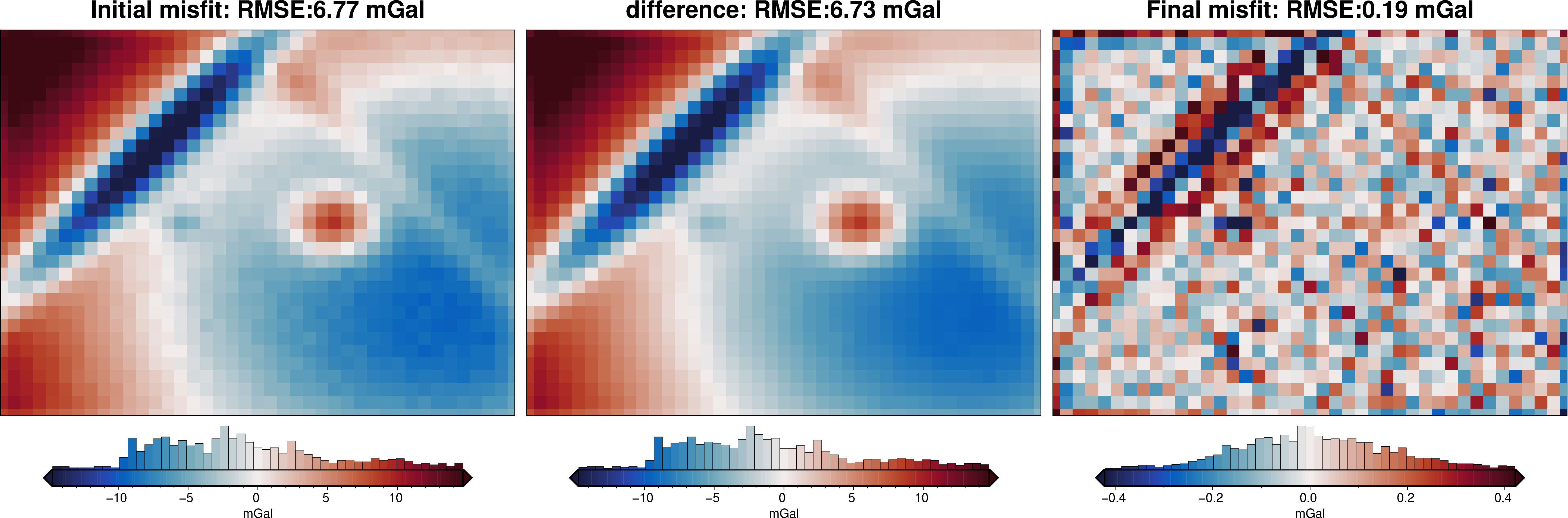
Gravity misfit

The gravity misfit is the difference between the observed gravity anomaly and the forward gravity of the starting topography.

The misfit can be separated into regional and residual components, here we assume the regional component is 0.

grav_df = regional.regional_separation(
    method="constant",
    constant=0,
    grav_df=grav_df,
)

grav_df.describe()

	northing	easting	upward	gravity_anomaly	starting_gravity	misfit	reg	res
count	1271.000000	1271.00000	1271.0	1271.000000	1271.0	1271.000000	1271.0	1271.000000
mean	15000.000000	20000.00000	1000.0	-0.868201	0.0	-0.868201	0.0	-0.868201
std	8947.792584	11836.81698	0.0	6.712766	0.0	6.712766	0.0	6.712766
min	0.000000	0.00000	1000.0	-17.194385	-0.0	-17.194385	0.0	-17.194385
25%	7000.000000	10000.00000	1000.0	-5.955907	-0.0	-5.955907	0.0	-5.955907
50%	15000.000000	20000.00000	1000.0	-1.790258	0.0	-1.790258	0.0	-1.790258
75%	23000.000000	30000.00000	1000.0	2.738776	-0.0	2.738776	0.0	2.738776
max	30000.000000	40000.00000	1000.0	18.024858	-0.0	18.024858	0.0	18.024858

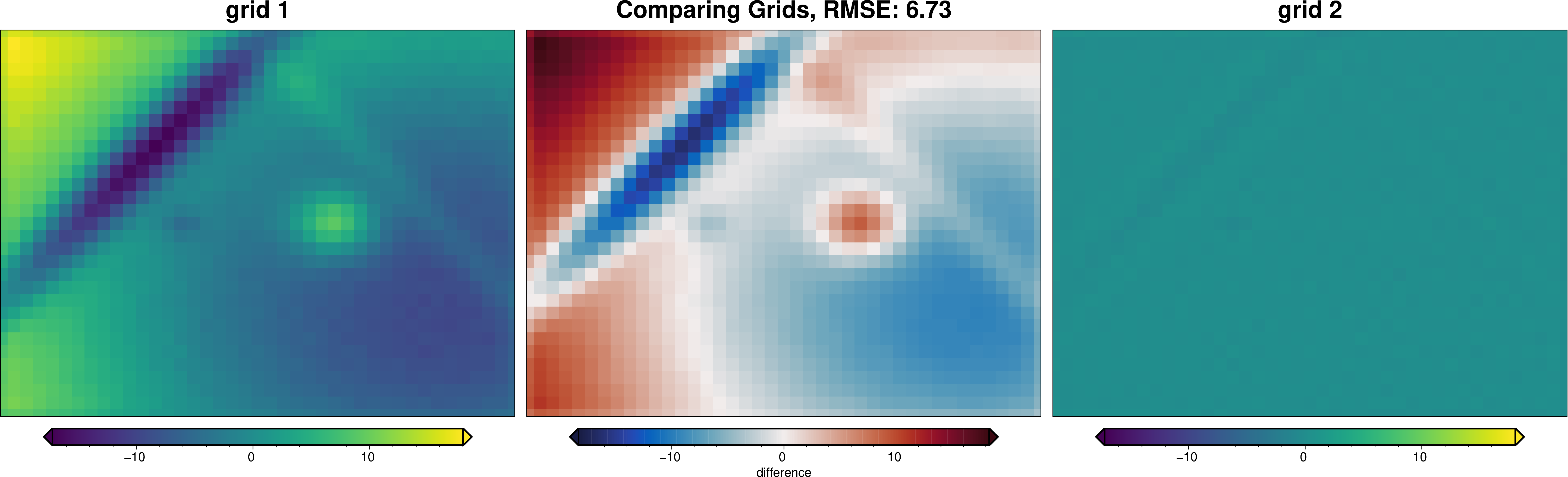
Plot the gravity anomalies

grav_grid = grav_df.set_index(["northing", "easting"]).to_xarray()

fig = maps.plot_grd(
    grav_grid.gravity_anomaly,
    fig_height=10,
    title="Topo free disturbance",
    cmap="viridis",
    hist=True,
    cbar_label="mGal",
    frame=["nSWe", "xaf10000", "yaf10000"],
)

fig = maps.plot_grd(
    grav_grid.starting_gravity,
    fig=fig,
    origin_shift="x",
    fig_height=10,
    title="Starting gravity",
    cmap="viridis",
    hist=True,
    cbar_label="mGal",
    frame=["nSwE", "xaf10000", "yaf10000"],
)


fig = maps.plot_grd(
    grav_grid.misfit,
    fig=fig,
    origin_shift="x",
    fig_height=10,
    title="Misfit",
    cmap="viridis",
    hist=True,
    cbar_label="mGal",
    frame=["nSwE", "xaf10000", "yaf10000"],
)

fig = maps.plot_grd(
    grav_grid.reg,
    fig=fig,
    origin_shift="x",
    fig_height=10,
    title="Regional misfit",
    cmap="viridis",
    hist=True,
    cbar_label="mGal",
    frame=["nSwE", "xaf10000", "yaf10000"],
)

fig = maps.plot_grd(
    grav_grid.res,
    fig=fig,
    origin_shift="x",
    fig_height=10,
    title="Residual misfit",
    cmap="balance+h0",
    hist=True,
    cbar_label="mGal",
    frame=["nSwE", "xaf10000", "yaf10000"],
)
fig.show()

makecpt [ERROR]: Option T: min >= max
makecpt [ERROR]: Option T: min >= max
makecpt [ERROR]: Option T: min >= max
makecpt [ERROR]: Option T: min >= max

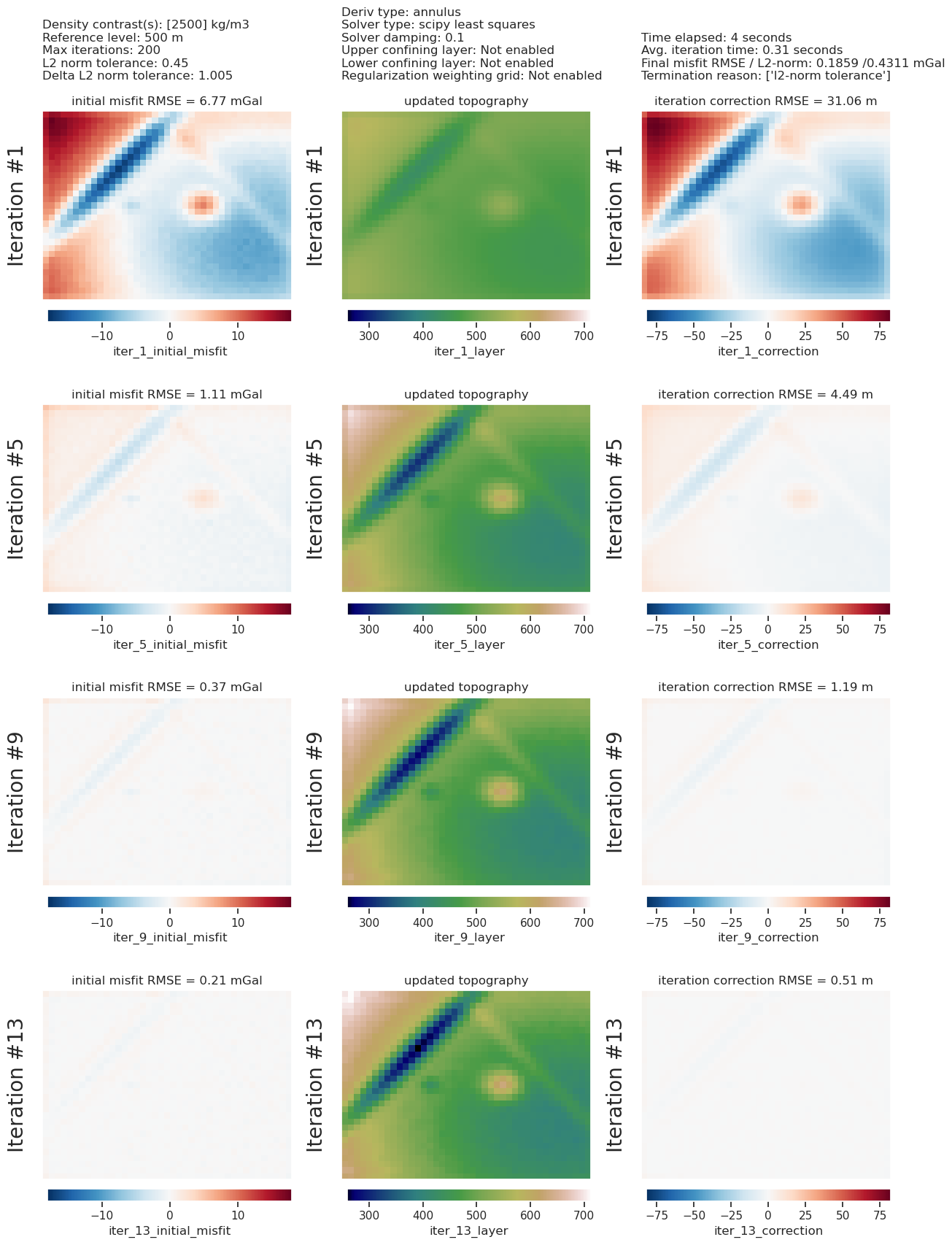
Perform inversion

Now that we have a starting model and residual gravity misfit data we can start the inversion.

# run the inversion
results = inversion.run_inversion(
    grav_df=grav_df,
    prism_layer=starting_prisms,
    solver_damping=0.1,
    # set stopping criteria
    max_iterations=200,
    l2_norm_tolerance=0.45,  # gravity error is .2 mGal, L2-norm is sqrt(mGal) so ~0.45
    delta_l2_norm_tolerance=1.005,
    plot_convergence=True,
)

# collect the results
topo_results, grav_results, parameters, elapsed_time = results

plotting.plot_inversion_results(
    grav_results,
    topo_results,
    parameters,
    region,
    iters_to_plot=4,
    plot_iter_results=True,
    plot_topo_results=True,
    plot_grav_results=True,
)

final_topography = topo_results.set_index(["northing", "easting"]).to_xarray().topo

_ = polar_utils.grd_compare(
    true_topography,
    final_topography,
    plot=True,
    grid1_name="True topography",
    grid2_name="Inverted topography",
    robust=True,
    hist=True,
    inset=False,
    verbose="q",
    title="difference",
    grounding_line=False,
    reverse_cpt=True,
    cmap="rain",
    diff_lims=(-20, 20),
)

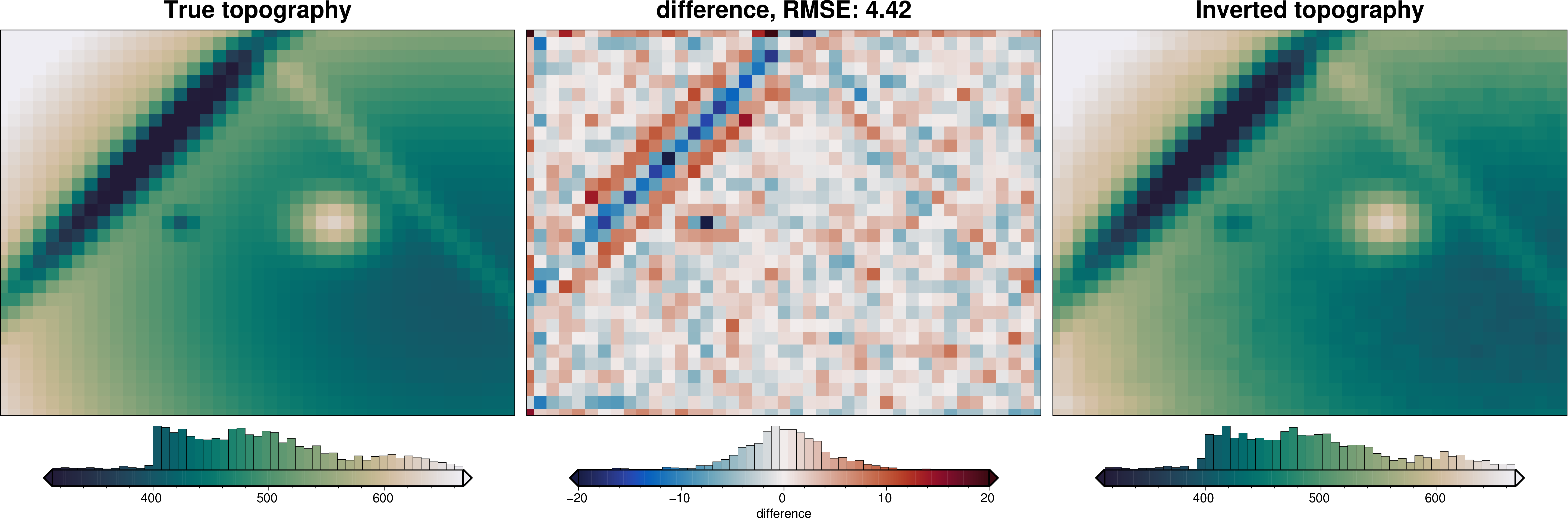
As you can see, the inversion successfully recovered the true topography. The root mean square difference between the true and recovered topography is low, but this is not too surprising since we gave the inversion the true density contrast and reference level values.