Variable density values#
Here we will extend the simple_inversion.ipynb example by using variable density contrast values. We create a map of density contrast values, and supply that instead of the constant density contrast value. This is useful for situations where you know the density contrast across your topographic layer is interest is variable, such as modelled the sediment-basement contact where the basement density changes regionally.
Import packages#
[1]:
%load_ext autoreload
%autoreload 2

import logging

import verde as vd
import xarray as xr
from polartoolkit import maps
from polartoolkit import utils as polar_utils

from invert4geom import inversion, plotting, regional, synthetic, utils

# set up logging to see what's going on
logging.basicConfig(level=logging.INFO)
Create observed gravity data#
To run the inversion, we need to have observed gravity data. In this simple example, we will first create a synthetic topography, which represents the true Earth topography which we hope to recover during the inverison. From this topography, we will create a layer of vertical right-rectangular prisms, which allows us to calculated the gravity effect of the topography. This will act as our observed gravity data.
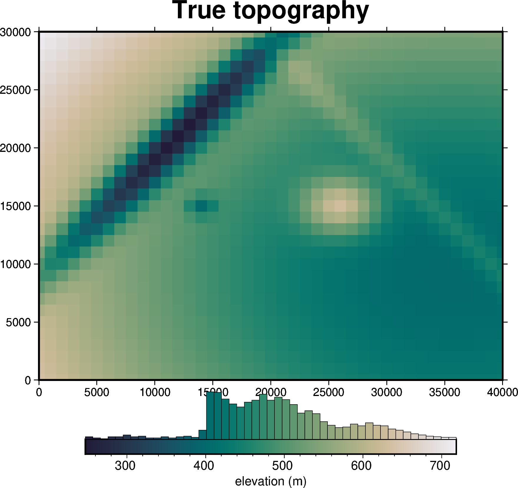
True topography#
[13]:
spacing = 1000
region = (0, 40000, 0, 30000)

true_topography, _, _, _ = synthetic.load_synthetic_model(
    spacing=spacing,
    region=region,
)

# plot the true topography
fig = maps.plot_grd(
    true_topography,
    fig_height=10,
    title="True topography",
    cmap="rain",
    hist=True,
    reverse_cpt=True,
    cbar_label="elevation (m)",
    frame=["nSWe", "xaf10000", "yaf10000"],
)
fig.show()

true_topography
[13]:
<xarray.DataArray 'upward' (northing: 31, easting: 41)> Size: 10kB
array([[637.12943453, 627.28784729, 617.55840384, ..., 428.39025144,
        429.33158321, 430.64751872],
       [632.95724141, 623.04617819, 613.24496334, ..., 422.67589466,
        423.6241977 , 424.94987872],
       [629.2139621 , 619.27333357, 609.41212904, ..., 417.59868139,
        418.55317844, 419.88752006],
       ...,
       [701.54094486, 692.82534357, 684.20926165, ..., 516.68829114,
        517.52190298, 518.68725132],
       [709.90739328, 701.33808009, 692.86661587, ..., 528.15742206,
        528.97704204, 530.12283044],
       [718.55151946, 710.13334959, 701.81130286, ..., 540.00720706,
        540.8123708 , 541.93795008]], shape=(31, 41))
Coordinates:
  * easting   (easting) float64 328B 0.0 1e+03 2e+03 ... 3.8e+04 3.9e+04 4e+04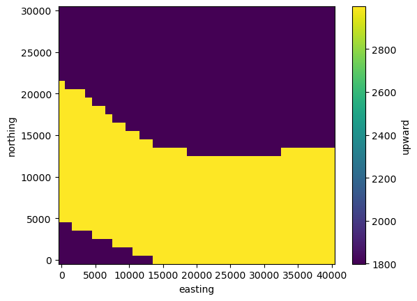
* northing (northing) float64 248B 0.0 1e+03 2e+03 ... 2.8e+04 2.9e+04 3e+04Density distribution#
[3]:
# create some random synthetic data
synthetic_data = synthetic.synthetic_topography_regional(
    spacing,
    region,
    yoffset=20,
)

# the first density contrast is between sediment (~2300 kg/m3) and air (~1 kg/m3)
density_contrast_1 = 1800 - 1

# the second density contrast is between crystalline basement (~2800 kg/m3) and air
# (~1 kg/m3)
density_contrast_2 = 3000 - 1

# use it to create a surface density distribution
density_dist = xr.where(synthetic_data > 0, density_contrast_1, density_contrast_2)

density_dist.plot()
[3]:
<matplotlib.collections.QuadMesh at 0x7f54f38c8f20>
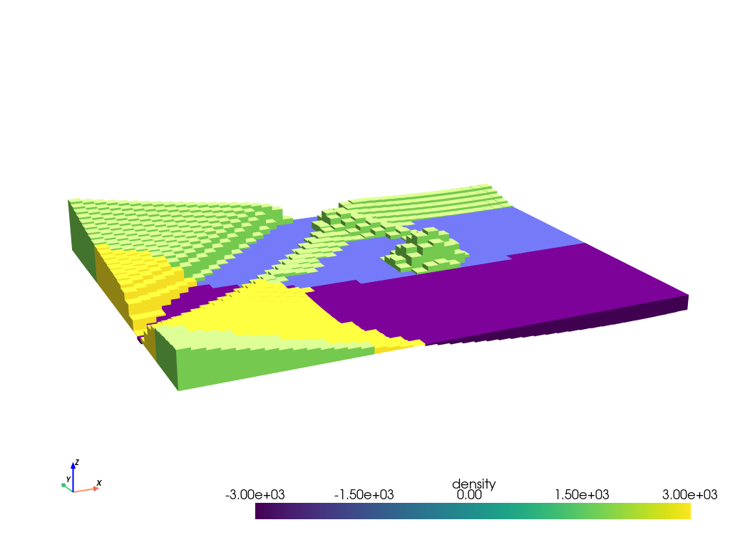
Prism layer#
[4]:
# prisms are created between the mean topography value and the height of the topography
zref = true_topography.values.mean()

# prisms above zref have positive density contrast and prisms below zref have negative
# density contrast
# density contrast values come from above density distribution
density_grid = xr.where(true_topography >= zref, density_dist, -density_dist)

# create layer of prisms
prisms = utils.grids_to_prisms(
    true_topography,
    zref,
    density=density_grid,
)

plotting.show_prism_layers(
    prisms,
    color_by="density",
    log_scale=False,
    zscale=20,
    backend="static",
)
Forward gravity of prism layer#
[5]:
# make pandas dataframe of locations to calculate gravity
# this represents the station locations of a gravity survey
# create lists of coordinates
coords = vd.grid_coordinates(
    region=region,
    spacing=spacing,
    pixel_register=False,
    extra_coords=1000,  # survey elevation
)

# grid the coordinates
observations = vd.make_xarray_grid(
    (coords[0], coords[1]),
    data=coords[2],
    data_names="upward",
    dims=("northing", "easting"),
).upward

grav_df = vd.grid_to_table(observations)

grav_df["grav"] = prisms.prism_layer.gravity(
    coordinates=(
        grav_df.easting,
        grav_df.northing,
        grav_df.upward,
    ),
    field="g_z",
    progressbar=True,
)

grav_df
[5]:
| northing | easting | upward | grav | |
|---|---|---|---|---|
| 0 | 0.0 | 0.0 | 1000.0 | 6.475985 |
| 1 | 0.0 | 1000.0 | 1000.0 | 7.085818 |
| 2 | 0.0 | 2000.0 | 1000.0 | 6.778545 |
| 3 | 0.0 | 3000.0 | 1000.0 | 6.331323 |
| 4 | 0.0 | 4000.0 | 1000.0 | 5.846485 |
| ... | ... | ... | ... | ... |
| 1266 | 30000.0 | 36000.0 | 1000.0 | 2.240682 |
| 1267 | 30000.0 | 37000.0 | 1000.0 | 2.239181 |
| 1268 | 30000.0 | 38000.0 | 1000.0 | 2.242789 |
| 1269 | 30000.0 | 39000.0 | 1000.0 | 2.219555 |
| 1270 | 30000.0 | 40000.0 | 1000.0 | 1.921481 |
1271 rows × 4 columns
[12]:
# contaminate gravity with 0.2 mGal of random noise
grav_df["gravity_anomaly"], stddev = synthetic.contaminate(
grav_df.grav,
stddev=0.2,
percent=False,
seed=0,
)
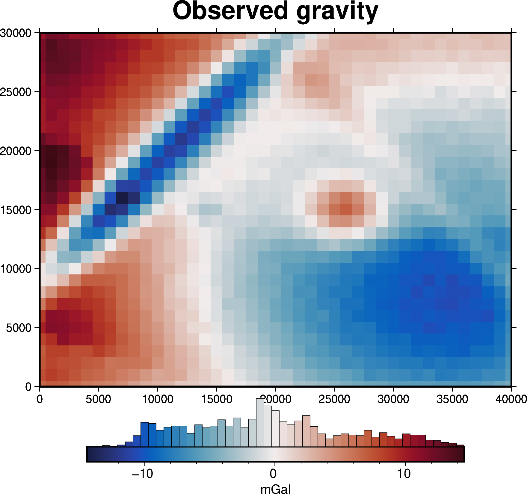
# plot the observed gravity
fig = maps.plot_grd(
grav_df.set_index(["northing", "easting"]).to_xarray().gravity_anomaly,
fig_height=10,
title="Observed gravity",
cmap="balance+h0",
hist=True,
cbar_label="mGal",
frame=["nSWe", "xaf10000", "yaf10000"],
)
fig.show()
Gravity misfit#
Now we need to create a starting model of the topography to start the inversion with. Since here we have no knowledge of either the topography or the appropriate reference level (zref), the starting model is flat, and therefore it’s forward gravity is 0. If you had a non-flat starting model, you would need to calculate it’s forward gravity effect, and subtract it from our observed gravity to get a starting gravity misfit.
In this simple case, we assume that we know the true density contrast and appropriate reference value for the topography (zref), and use these values to create our flat starting model. Note that in a real world scenario, these would be unknowns which would need to be carefully chosen, as explained in the following notebooks.
[7]:
# create flat topography grid with a constant height
starting_topography = xr.full_like(true_topography, zref)

# prisms are created between zref and the height of the topography, which for this
# starting model is flat.
# prisms above zref have positive density contrast and prisms below zref have negative
# density contrast
density_grid = xr.where(starting_topography >= zref, density_dist, -density_dist)

# create layer of prisms
starting_prisms = utils.grids_to_prisms(
    starting_topography,
    zref,
    density=density_grid,
)

# currently not working with flat layers
# plotting.show_prism_layers(
#     starting_prisms,
#     color_by="thickness",
#     log_scale=False,
#     zscale=20,
#     backend="static",
# )
starting_prisms.density.plot()
[7]:
<matplotlib.collections.QuadMesh at 0x7f5477b155e0>

[8]:
# since our starting model is flat, the starting gravity is 0
grav_df["starting_gravity"] = 0

# in many cases, we want to remove a regional signal from the misfit to isolate the
# residual signal. In this simple case, we assume there is no regional misfit and set
# it to 0
grav_df = regional.regional_separation(
    method="constant",
    constant=0,
    grav_df=grav_df,
)

grav_df.describe()
[8]:
| northing | easting | upward | grav | gravity_anomaly | starting_gravity | misfit | reg | res | |
|---|---|---|---|---|---|---|---|---|---|
| count | 1271.000000 | 1271.00000 | 1271.0 | 1271.000000 | 1271.000000 | 1271.0 | 1271.000000 | 1271.0 | 1271.000000 |
| mean | 15000.000000 | 20000.00000 | 1000.0 | -0.538567 | -0.538567 | 0.0 | -0.538567 | 0.0 | -0.538567 |
| std | 8947.792584 | 11836.81698 | 0.0 | 6.103569 | 6.102644 | 0.0 | 6.102644 | 0.0 | 6.102644 |
| min | 0.000000 | 0.00000 | 1000.0 | -14.071537 | -14.400686 | 0.0 | -14.400686 | 0.0 | -14.400686 |
| 25% | 7000.000000 | 10000.00000 | 1000.0 | -5.125926 | -5.057012 | 0.0 | -5.057012 | 0.0 | -5.057012 |
| 50% | 15000.000000 | 20000.00000 | 1000.0 | -0.901472 | -0.901253 | 0.0 | -0.901253 | 0.0 | -0.901253 |
| 75% | 23000.000000 | 30000.00000 | 1000.0 | 2.929567 | 2.964659 | 0.0 | 2.964659 | 0.0 | 2.964659 |
| max | 30000.000000 | 40000.00000 | 1000.0 | 14.726204 | 14.492359 | 0.0 | 14.492359 | 0.0 | 14.492359 |
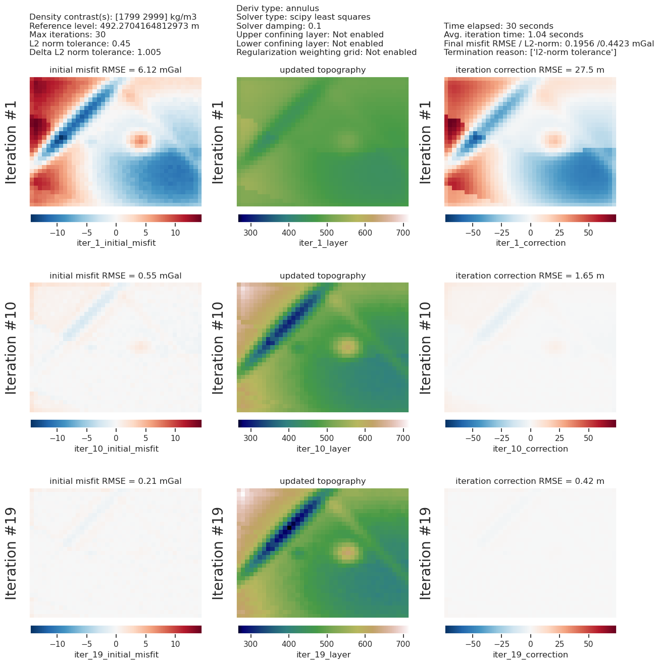
Perform inversion#
Now that we have a starting model and residual gravity misfit data we can start the inversion.
[9]:
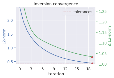
logging.getLogger().setLevel(logging.WARN)

# run the inversion
results = inversion.run_inversion(
    grav_df=grav_df,
    prism_layer=starting_prisms,
    solver_damping=0.1,
    # set stopping criteria
    max_iterations=30,
    l2_norm_tolerance=0.45,  # gravity error is .2 mGal, L2-norm is sqrt(mGal) so ~0.45
    delta_l2_norm_tolerance=1.005,
    #  display the convergence of the inversion
    plot_dynamic_convergence=True,
)

# collect the results
topo_results, grav_results, parameters, elapsed_time = results
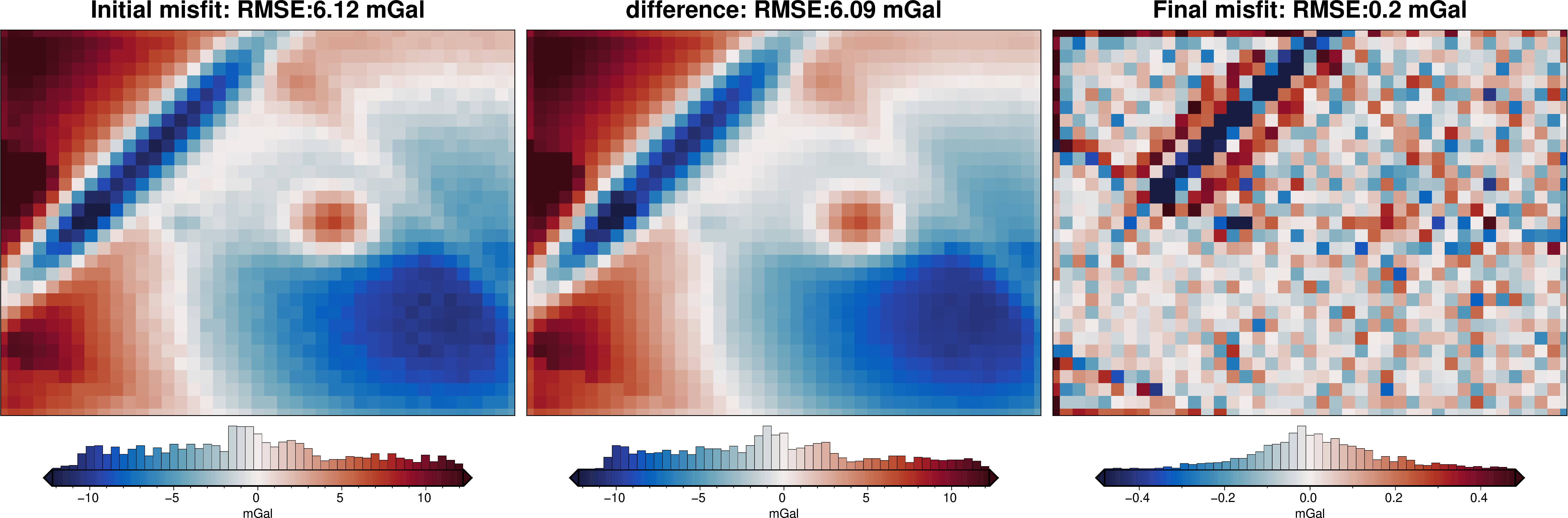
[10]:
plotting.plot_inversion_results(
    grav_results,
    topo_results,
    parameters,
    region,
    iters_to_plot=3,
    plot_iter_results=True,
    plot_topo_results=True,
    plot_grav_results=True,
)
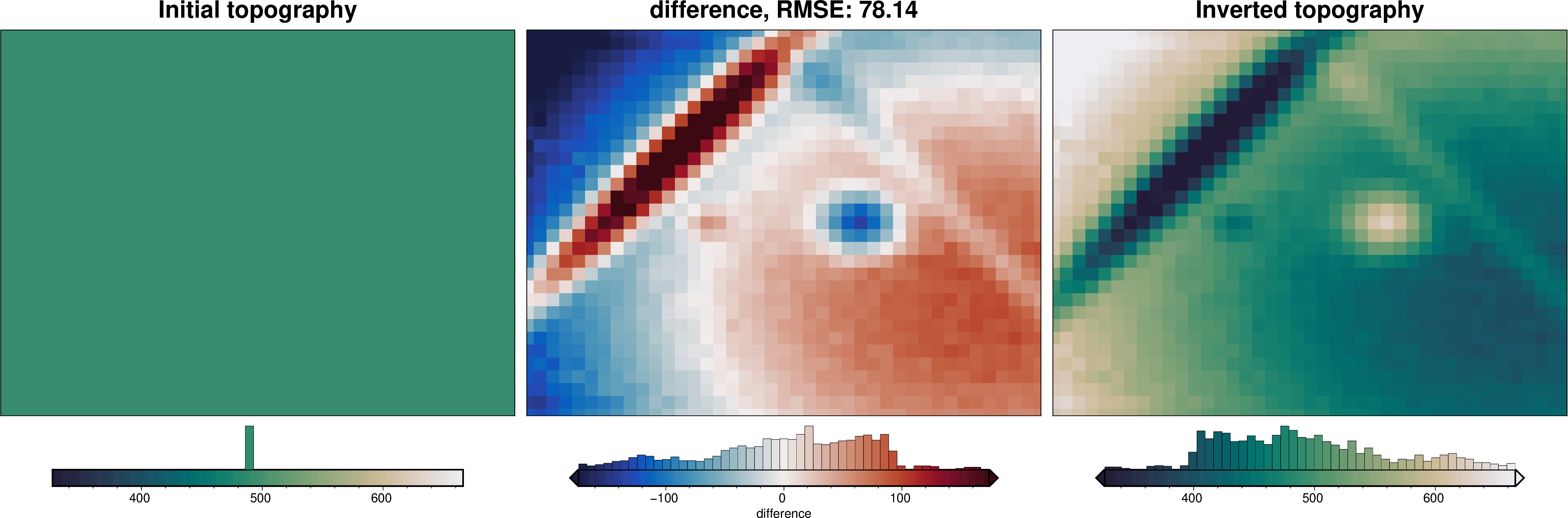
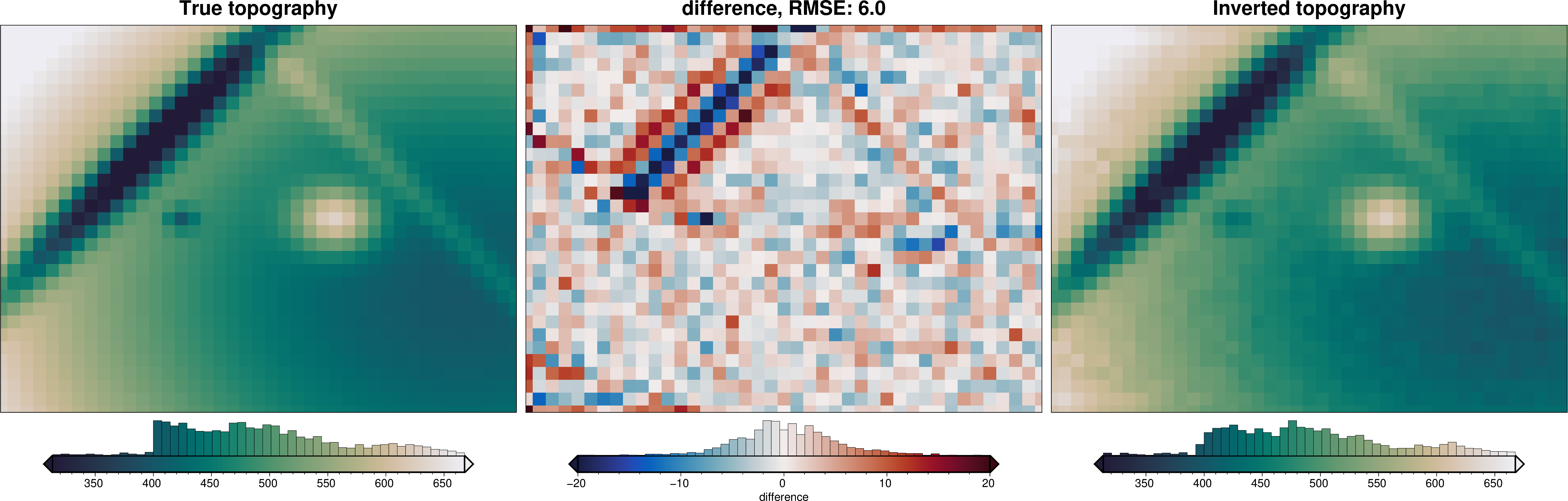
[11]:
final_topography = topo_results.set_index(["northing", "easting"]).to_xarray().topo

_ = polar_utils.grd_compare(
    true_topography,
    final_topography,
    # plot_type="xarray",
    plot=True,
    grid1_name="True topography",
    grid2_name="Inverted topography",
    robust=True,
    hist=True,
    inset=False,
    verbose="q",
    title="difference",
    grounding_line=False,
    reverse_cpt=True,
    cmap="rain",
    diff_lims=(-20, 20),
)