CRUST1 Moho Model from Uieda et al. 2017.#
Here we attempt to reproduce the CRUST1 Moho inversion for South America from Uieda et al. 2017: Fast nonlinear gravity inversion in spherical coordinates with application to the South American Moho. This is a semi-synthetic model, where true Moho topography data from CRUST1 is used to forward model the observed gravity. This synthetic gravity data is then used to invert for Moho topography. We start by following their approach, but using Invert4Geom. We follow this by using our own approach of incorporating a starting model and adhering to points of known Moho elevation.
[1]:
import os

import boule as bl
import numpy as np
import pandas as pd
import polartoolkit as ptk
import pooch
import pygmt
import verde as vd
import xarray as xr

import invert4geom

# set EPSG for plotting functions
os.environ["POLARTOOLKIT_EPSG"] = "4326"
/home/mdtanker/miniforge3/envs/invert4geom/lib/python3.12/site-packages/UQpy/__init__.py:6: UserWarning: pkg_resources is deprecated as an API. See https://setuptools.pypa.io/en/latest/pkg_resources.html. The pkg_resources package is slated for removal as early as 2025-11-30. Refrain from using this package or pin to Setuptools<81.
  import pkg_resources
Get datasets#
Here we use Pooch to download the CRUST1 global Moho topography dataset, and the locations of seismic measurements of Moho depth for South America. We perform some preprocessing on these datasets, subsetting them to match the geographic extent used in the paper.
[2]:
# download gridded CRUST1 Moho depth data
url = "https://igppweb.ucsd.edu/~gabi/crust1/depthtomoho.xyz.zip"
known_hash = "36089a537ed45795557999003d0eada9935f1cc589a6ddb486a7eac716dc7ff2"
path = pooch.retrieve(
    url=url,
    path=pooch.os_cache("invert4geom"),
    known_hash=known_hash,
    progressbar=True,
    processor=pooch.Unzip(),
)[0]

# read data
df = pd.read_csv(
    path, header=None, sep=r"\s+", names=["longitude", "latitude", "upward"]
)

# turn elevation to meters
df["upward"] = df.upward * 1000

# turn into grid
true_moho = (
    df.set_index(["latitude", "longitude"]).to_xarray().rio.write_crs("EPSG:4326")
)

# resample to lower resolution for speed
true_moho = true_moho.coarsen(longitude=2, latitude=2, boundary="trim").mean()

# subset to south america
region_ll = (-90, -30, -60, 20)
true_moho = true_moho.sel(
    longitude=slice(region_ll[0], region_ll[1]),
    latitude=slice(region_ll[2], region_ll[3]),
).drop_vars("spatial_ref")

info = ptk.get_grid_info(true_moho.upward)
spacing, region_ll = info[0], info[1]

true_moho
[2]:
<xarray.Dataset> Size: 10kB
Dimensions:    (latitude: 40, longitude: 30)
Coordinates:
  * latitude   (latitude) float64 320B -59.0 -57.0 -55.0 ... 15.0 17.0 19.0
  * longitude  (longitude) float64 240B -89.0 -87.0 -85.0 ... -35.0 -33.0 -31.0
Data variables:
upward (latitude, longitude) float64 10kB -1.2e+04 ... -1.182e+04[3]:
# download seismic point measures for Moho depths
url = "https://raw.githubusercontent.com/pinga-lab/paper-moho-inversion-tesseroids/master/data/crust1-point-depths.txt"
known_hash = "788426dbb100caf86b4973acf8e2b1964a2cfe517cb17c3ea9cd30ee99c9c6fb"
path = pooch.retrieve(
    url=url,
    path=pooch.os_cache("invert4geom"),
    known_hash=known_hash,
    progressbar=True,
)

# read data
df = pd.read_csv(path, skiprows=4, sep=" ", names=["latitude", "longitude", "upward"])

# subset to region
constraint_points = ptk.points_inside_region(
    df, region_ll, names=("longitude", "latitude")
)

# as in the paper, the depth values used are actually sampled from the CRUST1 model
constraint_points = invert4geom.sample_grids(
    constraint_points, true_moho.upward, "upward", coord_names=("longitude", "latitude")
)

constraint_points.describe()
[3]:
| latitude | longitude | upward | |
|---|---|---|---|
| count | 937.000000 | 937.000000 | 937.000000 |
| mean | -15.779085 | -60.878246 | -40561.803472 |
| std | 13.436299 | 12.894853 | 15101.721242 |
| min | -54.140000 | -86.300000 | -66766.186387 |
| 25% | -25.700000 | -70.346300 | -53906.545409 |
| 50% | -17.360000 | -66.780000 | -40197.550499 |
| 75% | -7.639000 | -47.794900 | -31783.398398 |
| max | 13.949700 | -35.104000 | -11317.005710 |
Convert elevations to be geocentric#
For this inversion, since it covers a large geographic region, we will use tesseroids, instead of prisms, for discretization. This accounts for the curvature of the Earth, an important consideration if your study site covers a large region. The tops and bottoms of prisms are defined to heights, typically relative to an ellipsoid model. However, for tesseroids, the tops and bottoms are defined by radii, typically from the center of an ellipsoid model. Due to this, we need to convert ellipsoidal heights to be relative to the center of the ellipsoid.
[4]:
# get the coordinates of the grid
_longitude, latitude = np.meshgrid(true_moho.longitude, true_moho.latitude)

# compute the geocentric radius at each latitude
geocentric_radius = bl.WGS84.geocentric_radius(latitude)

# add geocentric radius to the xarray dataset
true_moho = true_moho.assign(
    geocentric_radius=(("latitude", "longitude"), geocentric_radius)
)

true_moho
[4]:
<xarray.Dataset> Size: 20kB
Dimensions:            (latitude: 40, longitude: 30)
Coordinates:
  * latitude           (latitude) float64 320B -59.0 -57.0 -55.0 ... 17.0 19.0
  * longitude          (longitude) float64 240B -89.0 -87.0 ... -33.0 -31.0
Data variables:
    upward             (latitude, longitude) float64 10kB -1.2e+04 ... -1.182...
geocentric_radius (latitude, longitude) float64 10kB 6.362e+06 ... 6.376...[5]:
fig = pygmt.Figure()
proj = "M10c"
# plot true moho topography relative to ellipsoid
pygmt.makecpt(
    cmap="rain",
    reverse=True,
    series=(ptk.get_min_max(true_moho.upward)),
    background=True,
)
fig.grdimage(
    true_moho.upward,
    projection=proj,
    frame=["neSW+tMoho topography (ellipsoidal)", "af"],
)
fig.colorbar(frame="af+lelevation (m)", position="JCR")
fig.coast(shorelines="0.5p,black", borders=["1/0.5p,black"])

# plot seismic points
fig.plot(
    x=constraint_points.longitude,
    y=constraint_points.latitude,
    style="c.2c",
    fill=constraint_points.upward,
    cmap=True,
    pen=".6p,black",
)

fig.shift_origin(xshift="w+4c")

# plot geocentric radius
pygmt.makecpt(
    cmap="rain",
    reverse=True,
    series=(ptk.get_min_max(true_moho.geocentric_radius)),
    background=True,
)
fig.grdimage(
    true_moho.geocentric_radius,
    projection=proj,
    frame=["neSw+tGeocentric radius", "af"],
)
fig.colorbar(frame="af+lelevation (m)", position="JCR")
fig.coast(shorelines="0.5p,black", borders=["1/0.5p,black"])

fig.shift_origin(xshift="w+4c")

# plot true moho topography relative to center of the Earth
upward_geocentric = true_moho.upward + true_moho.geocentric_radius
pygmt.makecpt(
    cmap="rain",
    reverse=True,
    series=(ptk.get_min_max(upward_geocentric)),
    background=True,
)
fig.grdimage(
    upward_geocentric,
    projection=proj,
    frame=["neSw+tMoho topography (geocentric)", "af"],
)
fig.colorbar(frame="af+lelevation (m)", position="JCR")
fig.coast(shorelines="0.5p,black", borders=["1/0.5p,black"])

fig.show()

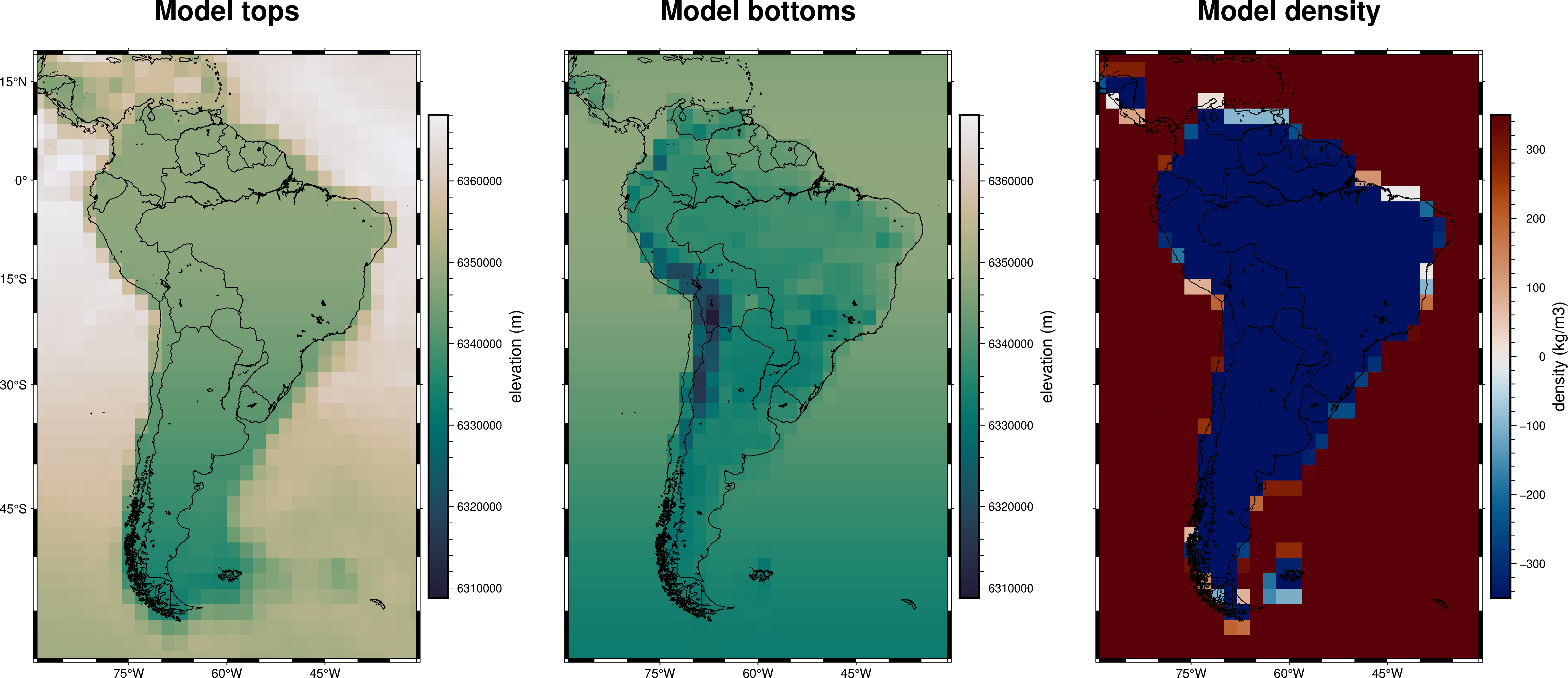
Create tesseroid model#
[6]:
# Define the reference level (height in meters).
# This is the Moho depth of the Normal Earth
true_zref = -30e3

# The density contrast is negative if the relief is below the reference
true_density_contrast = 350

# make tesseroid layer
true_model = invert4geom.create_model(
    zref=true_zref,
    density_contrast=true_density_contrast,
    topography=true_moho,
    model_type="tesseroids",
)
true_model
[6]:
<xarray.Dataset> Size: 97kB
Dimensions:                (latitude: 40, longitude: 30)
Coordinates:
  * latitude               (latitude) float64 320B -59.0 -57.0 ... 17.0 19.0
  * longitude              (longitude) float64 240B -89.0 -87.0 ... -33.0 -31.0
    top                    (latitude, longitude) float64 10kB 6.35e+06 ... 6....
    bottom                 (latitude, longitude) float64 10kB 6.332e+06 ... 6...
Data variables:
    density                (latitude, longitude) int64 10kB 350 350 ... 350 350
    thickness              (latitude, longitude) float64 10kB 1.8e+04 ... 1.8...
    starting_topography    (latitude, longitude) float64 10kB -1.2e+04 ... -1...
    topography             (latitude, longitude) float64 10kB -1.2e+04 ... -1...
    mask                   (latitude, longitude) float64 10kB 1.0 1.0 ... 1.0
    geocentric_radius      (latitude, longitude) float64 10kB 6.362e+06 ... 6...
    upper_confining_layer  (latitude, longitude) float64 10kB nan nan ... nan
    lower_confining_layer  (latitude, longitude) float64 10kB nan nan ... nan
Attributes:
    zref:              -30000.0
    density_contrast:  350
    region:            (-89.0, -31.0, -59.0, 19.0)
    spacing:           2.0
    buffer_width:      0
    inner_region:      (-89.0, -31.0, -59.0, 19.0)
    dataset_type:      model
    model_type:        tesseroids
coord_names: ('longitude', 'latitude')[7]:
fig = pygmt.Figure()
proj = "M10c"

# plot tesseroid tops
pygmt.makecpt(
    cmap="rain",
    reverse=True,
    series=(ptk.get_combined_min_max((true_model.top, true_model.bottom))),
    background=True,
)
fig.grdimage(true_model.top, projection=proj, frame=["neSW+tModel tops", "af"])
fig.colorbar(frame="af+lelevation (m)", position="JCR")
fig.coast(shorelines="0.5p,black", borders=["1/0.5p,black"])

fig.shift_origin(xshift="w+4c")

# plot tesseroid bottoms
fig.grdimage(true_model.bottom, projection=proj, frame=["neSw+tModel bottoms", "af"])
fig.colorbar(frame="af+lelevation (m)", position="JCR")
fig.coast(shorelines="0.5p,black", borders=["1/0.5p,black"])

fig.shift_origin(xshift="w+4c")

# # plot tesseroid densities
pygmt.makecpt(
    cmap="vik",
    background=True,
    series=ptk.get_min_max(true_model.density),
)
fig.grdimage(true_model.density, projection=proj, frame=["neSw+tModel density", "af"])
fig.colorbar(frame="af+ldensity (kg/m3)", position="JCR")
fig.coast(shorelines="0.5p,black", borders=["1/0.5p,black"])

fig.show()
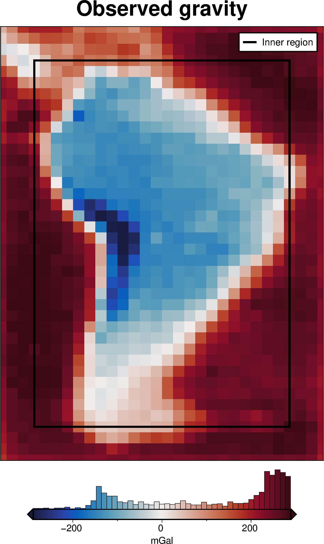
Observed gravity data#
We can now forward-model the effects of this moho model and add some noise to make a synthetic observed gravity dataset.
[8]:
# make pandas dataframe of locations to calculate gravity
# this represents the station locations of a gravity survey
# create lists of coordinates
coords = vd.grid_coordinates(
    region=true_model.region,
    spacing=true_model.spacing,
    pixel_register=False,
    extra_coords=50e3,  # survey elevation, ellipsoidal
)

# grid the coordinates
observations = vd.make_xarray_grid(
    (coords[0], coords[1]),
    data=coords[2],
    data_names="upward",
    dims=("latitude", "longitude"),
)

# get the coordinates of the grid
_longitude, latitude = np.meshgrid(observations.longitude, observations.latitude)

# compute the geocentric radius at each latitude
geocentric_radius = bl.WGS84.geocentric_radius(latitude)

# add geocentric radius to the xarray dataset
observations = observations.assign(
    geocentric_radius=(("latitude", "longitude"), geocentric_radius)
)

grav_data = invert4geom.create_data(
    observations,
    model_type="tesseroids",
)

grav_data.inv.forward_gravity(true_model, "gravity_anomaly")

# contaminate gravity with 5 mGal random noise
grav_data["gravity_anomaly"], stddev = invert4geom.contaminate(
    grav_data.gravity_anomaly,
    stddev=5,
    percent=False,
    seed=0,
)

grav_data
[8]:
<xarray.Dataset> Size: 29kB
Dimensions:            (latitude: 40, longitude: 30)
Coordinates:
  * latitude           (latitude) float64 320B -59.0 -57.0 -55.0 ... 17.0 19.0
  * longitude          (longitude) float64 240B -89.0 -87.0 ... -33.0 -31.0
Data variables:
    upward             (latitude, longitude) float64 10kB 5e+04 5e+04 ... 5e+04
    geocentric_radius  (latitude, longitude) float64 10kB 6.362e+06 ... 6.376...
    gravity_anomaly    (latitude, longitude) float64 10kB 178.8 213.2 ... 194.5
Attributes:
    region:        (-89.0, -31.0, -59.0, 19.0)
    spacing:       2.0
    buffer_width:  6.0
    inner_region:  (-83.0, -37.0, -53.0, 13.0)
    dataset_type:  data
    model_type:    tesseroids
coord_names: ('longitude', 'latitude')[9]:
grav_data.inv.plot_observed()
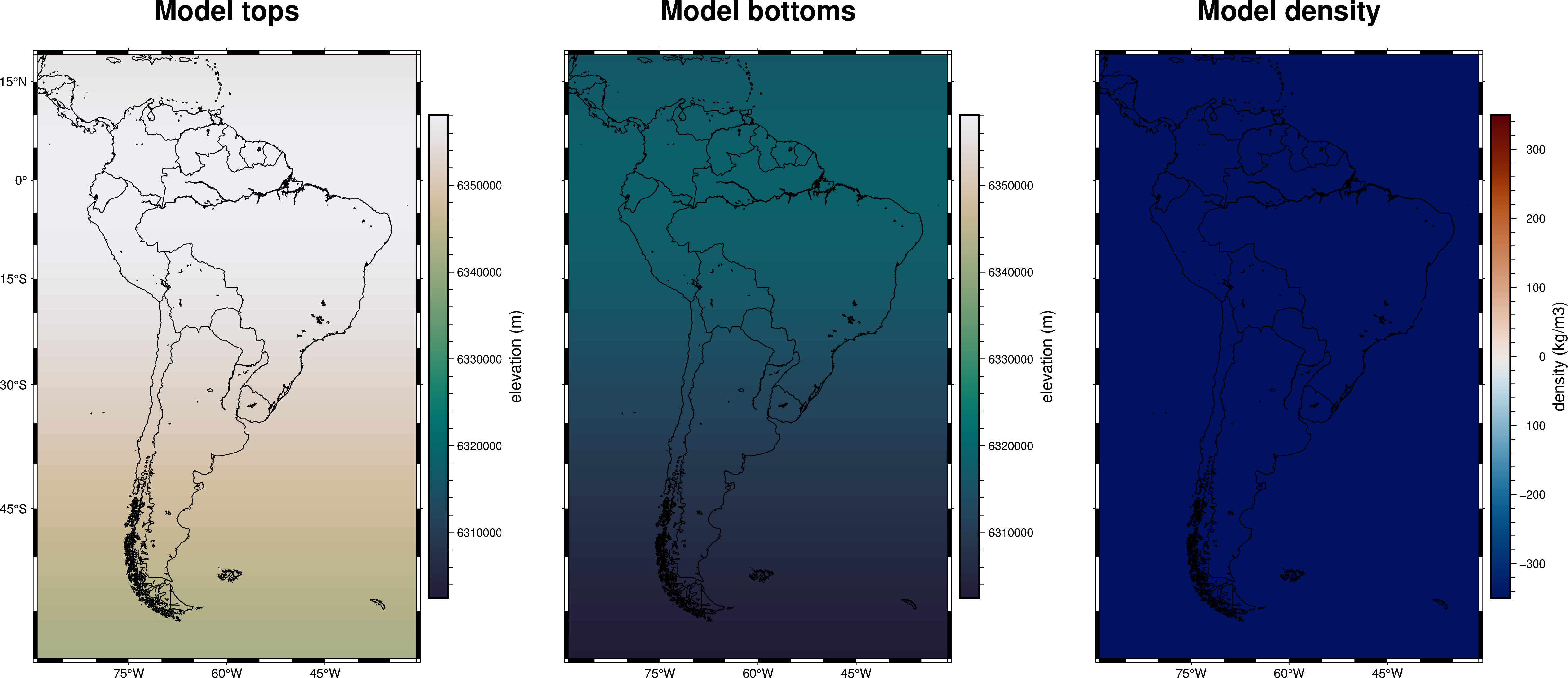
Starting model#
Following the paper’s approach, we create a starting model which is a flat layer at 60 km depth, with a reference level of -20 km and a density contrast of 500 kg/m3. This is used during the damping parameter cross-validation.
[10]:
# create flat topography grid
starting_topography = xr.full_like(true_moho.upward, -60e3).to_dataset(name="upward")

starting_topography["geocentric_radius"] = true_moho.geocentric_radius

# create initial model
model = invert4geom.create_model(
    zref=-20e3,
    density_contrast=500,
    topography=starting_topography,
    model_type="tesseroids",
    upper_confining_layer=xr.full_like(starting_topography.upward, 0),
)
model
[10]:
<xarray.Dataset> Size: 97kB
Dimensions:                (latitude: 40, longitude: 30)
Coordinates:
  * latitude               (latitude) float64 320B -59.0 -57.0 ... 17.0 19.0
  * longitude              (longitude) float64 240B -89.0 -87.0 ... -33.0 -31.0
    top                    (latitude, longitude) float64 10kB 6.342e+06 ... 6...
    bottom                 (latitude, longitude) float64 10kB 6.302e+06 ... 6...
Data variables:
    density                (latitude, longitude) int64 10kB -500 -500 ... -500
    thickness              (latitude, longitude) float64 10kB 4e+04 ... 4e+04
    starting_topography    (latitude, longitude) float64 10kB -6e+04 ... -6e+04
    topography             (latitude, longitude) float64 10kB -6e+04 ... -6e+04
    mask                   (latitude, longitude) float64 10kB 1.0 1.0 ... 1.0
    geocentric_radius      (latitude, longitude) float64 10kB 6.362e+06 ... 6...
    upper_confining_layer  (latitude, longitude) float64 10kB 0.0 0.0 ... 0.0
    lower_confining_layer  (latitude, longitude) float64 10kB nan nan ... nan
Attributes:
    zref:              -20000.0
    density_contrast:  500
    region:            (-89.0, -31.0, -59.0, 19.0)
    spacing:           2.0
    buffer_width:      0
    inner_region:      (-89.0, -31.0, -59.0, 19.0)
    dataset_type:      model
    model_type:        tesseroids
coord_names: ('longitude', 'latitude')[11]:
fig = pygmt.Figure()
proj = "M10c"

# plot tesseroid tops
pygmt.makecpt(
    cmap="rain",
    reverse=True,
    series=(ptk.get_combined_min_max((model.top, model.bottom))),
    background=True,
)
fig.grdimage(model.top, projection=proj, frame=["neSW+tModel tops", "af"])
fig.colorbar(frame="af+lelevation (m)", position="JCR")
fig.coast(shorelines="0.5p,black", borders=["1/0.5p,black"])

fig.shift_origin(xshift="w+4c")

# plot tesseroid bottoms
fig.grdimage(model.bottom, projection=proj, frame=["neSw+tModel bottoms", "af"])
fig.colorbar(frame="af+lelevation (m)", position="JCR")
fig.coast(shorelines="0.5p,black", borders=["1/0.5p,black"])

fig.shift_origin(xshift="w+4c")

# # plot tesseroid densities
pygmt.makecpt(
    cmap="vik+h0",
    background=True,
    series=[-350, 350],
)
fig.grdimage(model.density, projection=proj, frame=["neSw+tModel density", "af"])
fig.colorbar(frame="af+ldensity (kg/m3)", position="JCR")
fig.coast(shorelines="0.5p,black", borders=["1/0.5p,black"])

fig.show()
[12]:
# calculate the forward gravity of the initial model
grav_data.inv.forward_gravity(
    model,
    progressbar=True,
)
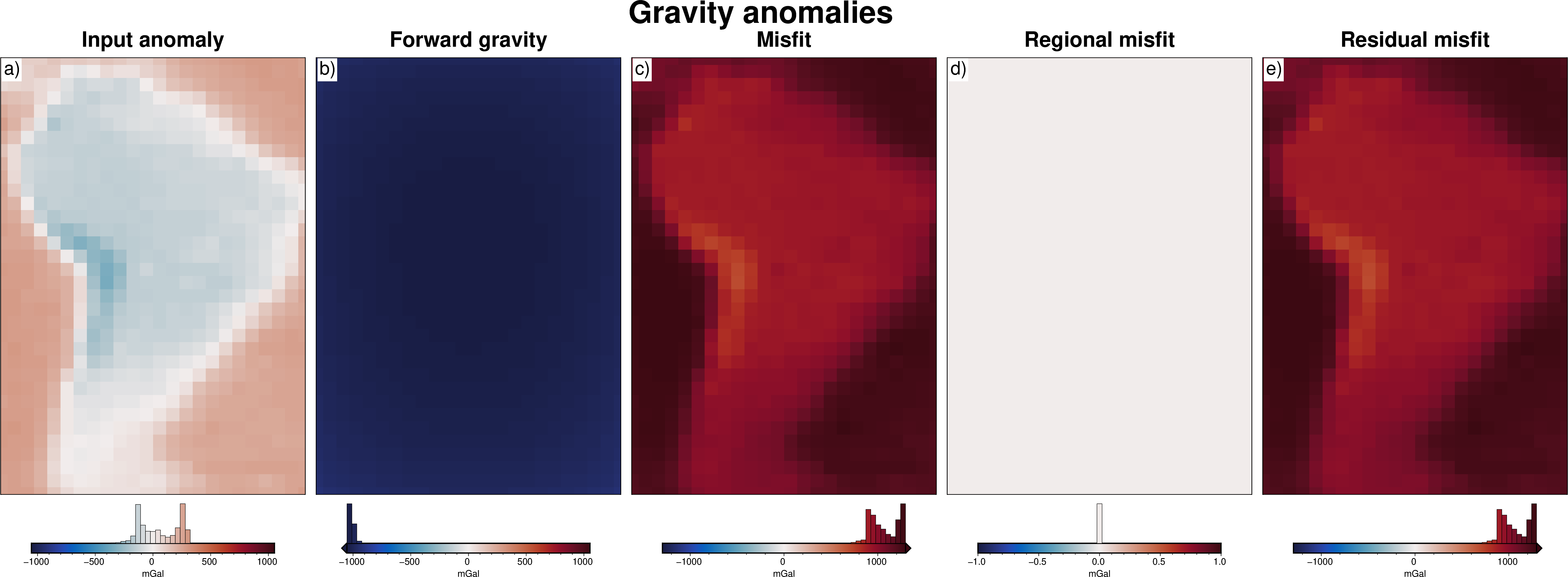
[13]:
# in many cases, we want to remove a regional signal from the misfit to isolate the
# residual signal. In this simple case, we assume there is no regional misfit and set
# it to 0
grav_data.inv.regional_separation(
    method="constant",
    constant=0,
)
grav_data.inv.plot_anomalies()
grav_data.inv.df
makecpt [ERROR]: Option T: min >= max
[13]:
| latitude | longitude | upward | geocentric_radius | gravity_anomaly | forward_gravity | misfit | reg | res | starting_forward_gravity | starting_misfit | starting_reg | starting_res | |
|---|---|---|---|---|---|---|---|---|---|---|---|---|---|
| 0 | -59.0 | -89.0 | 50000.0 | 6.362460e+06 | 178.806597 | -596.796560 | 775.603157 | 0.0 | 775.603157 | -596.796560 | 775.603157 | 0.0 | 775.603157 |
| 1 | -59.0 | -87.0 | 50000.0 | 6.362460e+06 | 213.223638 | -713.596725 | 926.820363 | 0.0 | 926.820363 | -713.596725 | 926.820363 | 0.0 | 926.820363 |
| 2 | -59.0 | -85.0 | 50000.0 | 6.362460e+06 | 226.627172 | -751.352163 | 977.979335 | 0.0 | 977.979335 | -751.352163 | 977.979335 | 0.0 | 977.979335 |
| 3 | -59.0 | -83.0 | 50000.0 | 6.362460e+06 | 227.875993 | -769.400419 | 997.276412 | 0.0 | 997.276412 | -769.400419 | 997.276412 | 0.0 | 997.276412 |
| 4 | -59.0 | -81.0 | 50000.0 | 6.362460e+06 | 226.983132 | -780.304951 | 1007.288083 | 0.0 | 1007.288083 | -780.304951 | 1007.288083 | 0.0 | 1007.288083 |
| ... | ... | ... | ... | ... | ... | ... | ... | ... | ... | ... | ... | ... | ... |
| 1195 | 19.0 | -39.0 | 50000.0 | 6.375887e+06 | 232.714938 | -793.011666 | 1025.726604 | 0.0 | 1025.726604 | -793.011666 | 1025.726604 | 0.0 | 1025.726604 |
| 1196 | 19.0 | -37.0 | 50000.0 | 6.375887e+06 | 230.113213 | -785.036334 | 1015.149547 | 0.0 | 1015.149547 | -785.036334 | 1015.149547 | 0.0 | 1015.149547 |
| 1197 | 19.0 | -35.0 | 50000.0 | 6.375887e+06 | 228.485861 | -772.889704 | 1001.375565 | 0.0 | 1001.375565 | -772.889704 | 1001.375565 | 0.0 | 1001.375565 |
| 1198 | 19.0 | -33.0 | 50000.0 | 6.375887e+06 | 225.113264 | -749.107926 | 974.221190 | 0.0 | 974.221190 | -749.107926 | 974.221190 | 0.0 | 974.221190 |
| 1199 | 19.0 | -31.0 | 50000.0 | 6.375887e+06 | 194.539430 | -657.844831 | 852.384260 | 0.0 | 852.384260 | -657.844831 | 852.384260 | 0.0 | 852.384260 |
1200 rows × 13 columns
Damping parameter cross validation#
[14]:
# setup the inversion
inv = invert4geom.Inversion(
    grav_data,
    model,
    deriv_type="finite_difference",
    # solver_damping=1e-3,
    # set stopping criteria
    max_iterations=20,
    l2_norm_tolerance=0.2,
    delta_l2_norm_tolerance=1.02,
)
[15]:
# inv.invert(plot_dynamic_convergence=True)
[16]:
# resample data at 1/2 spacing to include test points for cross-validation
inv.data = invert4geom.add_test_points(inv.data)
inv.data.inv.df
[16]:
| latitude | longitude | test | upward | geocentric_radius | gravity_anomaly | forward_gravity | misfit | reg | res | starting_forward_gravity | starting_misfit | starting_reg | starting_res | |
|---|---|---|---|---|---|---|---|---|---|---|---|---|---|---|
| 0 | -59.0 | -89.0 | False | 50000.0 | 6362460.0 | 178.806595 | -596.796570 | 775.603149 | 0.0 | 775.603149 | -596.796570 | 775.603149 | 0.0 | 775.603149 |
| 1 | -59.0 | -88.0 | True | 50000.0 | 6362460.0 | 197.328458 | -660.136951 | 857.465405 | 0.0 | 857.465405 | -660.136951 | 857.465405 | 0.0 | 857.465405 |
| 2 | -59.0 | -87.0 | False | 50000.0 | 6362460.0 | 213.223633 | -713.596741 | 926.820374 | 0.0 | 926.820374 | -713.596741 | 926.820374 | 0.0 | 926.820374 |
| 3 | -59.0 | -86.0 | True | 50000.0 | 6362460.0 | 221.998413 | -738.646454 | 960.644848 | 0.0 | 960.644848 | -738.646454 | 960.644848 | 0.0 | 960.644848 |
| 4 | -59.0 | -85.0 | False | 50000.0 | 6362460.0 | 226.627167 | -751.352173 | 977.979309 | 0.0 | 977.979309 | -751.352173 | 977.979309 | 0.0 | 977.979309 |
| ... | ... | ... | ... | ... | ... | ... | ... | ... | ... | ... | ... | ... | ... | ... |
| 4656 | 19.0 | -35.0 | False | 50000.0 | 6375887.5 | 228.485855 | -772.889709 | 1001.375549 | 0.0 | 1001.375549 | -772.889709 | 1001.375549 | 0.0 | 1001.375549 |
| 4657 | 19.0 | -34.0 | True | 50000.0 | 6375887.5 | 228.608715 | -765.943588 | 994.552303 | 0.0 | 994.552303 | -765.943588 | 994.552303 | 0.0 | 994.552303 |
| 4658 | 19.0 | -33.0 | False | 50000.0 | 6375887.5 | 225.113266 | -749.107910 | 974.221191 | 0.0 | 974.221191 | -749.107910 | 974.221191 | 0.0 | 974.221191 |
| 4659 | 19.0 | -32.0 | True | 50000.0 | 6375887.5 | 211.526425 | -707.693958 | 919.220394 | 0.0 | 919.220394 | -707.693958 | 919.220394 | 0.0 | 919.220394 |
| 4660 | 19.0 | -31.0 | False | 50000.0 | 6375887.5 | 194.539429 | -657.844849 | 852.384277 | 0.0 | 852.384277 | -657.844849 | 852.384277 | 0.0 | 852.384277 |
4661 rows × 14 columns
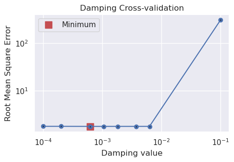
[17]:
damping_cv_obj = inv.optimize_inversion_damping(
    damping_limits=(1e-4, 1e-1),
    n_trials=8,
    plot_scores=True,
    fname="../tmp/uieda_CRUST1_damping_CV",
)
inv.solver_damping
Inversion terminated due to max_iterations limit. Consider increasing this limit.
[17]:
0.0006180487022349518
[18]:
damping_cv_obj.study.trials_dataframe().sort_values("value")
[18]:
| number | value | datetime_start | datetime_complete | duration | params_damping | user_attrs_fname | system_attrs_fixed_params | system_attrs_gp:relative_params:0 | state | |
|---|---|---|---|---|---|---|---|---|---|---|
| 6 | 6 | 1.760472 | 2026-07-13 14:25:47.874600 | 2026-07-13 14:25:53.075153 | 0 days 00:00:05.200553 | 0.000618 | ../tmp/uieda_CRUST1_damping_CV_trial_6 | NaN | {"damping": 0.0006180487022349518} | COMPLETE |
| 7 | 7 | 1.760647 | 2026-07-13 14:25:53.075772 | 2026-07-13 14:25:57.975511 | 0 days 00:00:04.899739 | 0.001059 | ../tmp/uieda_CRUST1_damping_CV_trial_7 | NaN | {"damping": 0.0010591559910431629} | COMPLETE |
| 4 | 4 | 1.761281 | 2026-07-13 14:25:35.816394 | 2026-07-13 14:25:40.762456 | 0 days 00:00:04.946062 | 0.001818 | ../tmp/uieda_CRUST1_damping_CV_trial_4 | NaN | {"damping": 0.001818096515449516} | COMPLETE |
| 5 | 5 | 1.761400 | 2026-07-13 14:25:40.763193 | 2026-07-13 14:25:47.873975 | 0 days 00:00:07.110782 | 0.003714 | ../tmp/uieda_CRUST1_damping_CV_trial_5 | NaN | {"damping": 0.0037135346405010924} | COMPLETE |
| 3 | 3 | 1.762450 | 2026-07-13 14:25:26.980311 | 2026-07-13 14:25:35.810887 | 0 days 00:00:08.830576 | 0.006271 | ../tmp/uieda_CRUST1_damping_CV_trial_3 | NaN | NaN | COMPLETE |
| 0 | 0 | 1.765479 | 2026-07-13 14:24:51.777426 | 2026-07-13 14:24:56.852986 | 0 days 00:00:05.075560 | 0.000100 | ../tmp/uieda_CRUST1_damping_CV_trial_0 | {'damping': 0.0001} | NaN | COMPLETE |
| 2 | 2 | 1.765510 | 2026-07-13 14:25:23.342028 | 2026-07-13 14:25:26.979716 | 0 days 00:00:03.637688 | 0.000198 | ../tmp/uieda_CRUST1_damping_CV_trial_2 | NaN | NaN | COMPLETE |
| 1 | 1 | 306.224502 | 2026-07-13 14:24:56.853620 | 2026-07-13 14:25:23.341451 | 0 days 00:00:26.487831 | 0.100000 | ../tmp/uieda_CRUST1_damping_CV_trial_1 | {'damping': 0.1} | NaN | COMPLETE |
The above plot shows the results of the damping parameter cross validation, and is equivalent to Figure 7a in the paper. The main difference is that we use a optimization approach instead of a grid search. This allows us to find the best value in fewer trials, as the parameter search space is quickly narrowed down. We performed 8 trials, compared to the 16 trials used in the paper.
Plot results#
[19]:
inv.plot_convergence()

inv.plot_inversion_results(
    iters_to_plot=2,
    fig_height=16,
)
[20]:
_ = ptk.grid_compare(
    true_moho.upward,
    inv.model.topography,
    region=inv.model.inner_region,
    grid1_name="True Moho",
    grid2_name="Inverted Moho",
    hist=True,
    inset=False,
    title="difference",
    reverse_cpt=True,
    cmap="rain",
    coast=True,
    coast_version="gmt",
)
[21]:
# sample the inverted topography at the constraint points
constraint_points = invert4geom.sample_grids(
    constraint_points,
    inv.model.topography,
    "inverted_topography",
    coord_names=("longitude", "latitude"),
)

constraint_points["inversion_error"] = (
    constraint_points.upward - constraint_points.inverted_topography
)
rmse = invert4geom.rmse(constraint_points.inversion_error)
print(f"RMSE: {rmse:.2f} m")
RMSE: 14647.85 m
Density / Reference level optimization#
Now that we have a optimal damping value, we can perform an optimization to find the optimal values for density contrast and reference level. For these, we pick a range of possible values, and perform a hyperparameter optimization to find the best set of values.
[22]:
inv.reinitialize_inversion()
[23]:
# run the optimization for the zref and density
density_zref_optimization_obj = inv.optimize_inversion_zref_density_contrast(
    constraints_df=constraint_points,
    zref_limits=(-35e3, -20e3),
    density_contrast_limits=(200, 500),
    n_trials=16,
    regional_grav_kwargs={
        "method": "constant",
        "constant": 0,
    },
    starting_topography_kwargs=dict(
        method="flat",
    ),
    plot_scores=True,
    fname="../tmp/uieda_CRUST1_zref_density_optimization",
)
'forward_gravity' already a variable of `grav_ds`, but is being overwritten since calculate_starting_gravity is True
'reg' already a column of `grav_df`, but is being overwritten since calculate_regional_misfit is True
[24]:
best_zref = density_zref_optimization_obj.study.best_params.get("zref")
best_density_contrast = density_zref_optimization_obj.study.best_params.get(
    "density_contrast"
)

print(f"Optimal zref: {best_zref / 1e3:.1f} km")
print(f"True zref: {true_zref / 1e3:.1f} km")
print(f"Optimal density contrast: {best_density_contrast:.1f} kg/m³")
print(f"True density contrast: {true_density_contrast:.1f} kg/m³")
Optimal zref: -30.3 km
True zref: -30.0 km
Optimal density contrast: 354.0 kg/m³
True density contrast: 350.0 kg/m³
[25]:
# we can also access the optimally-determined values through the `inv` object
print(f"Solver damping: {inv.solver_damping}")
print(f"Zref: {inv.model.zref / 1e3:.1f} km")
print(f"Density contrast: {inv.model.density_contrast:.1f} kg/m³")
Solver damping: 0.0006180487022349518
Zref: -30.3 km
Density contrast: 354.0 kg/m³
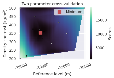
The above plot shows the results of the cross validation and is equivalent to Figure 7b in the paper. The optimal values they report are roughly the same as the true values (zref = 30 km and density contrast = 350 kg/m-3). The main difference is that they used a grid-search approach, testing evenly-spaced values between -35 and -20 km, and between 500 and 200 kg/m-3. We instead used an optimization approach, where the parameters space is smartly searched based on the scores of the past trials. As you can see, this allows us to find the optimal values in far fewer trials. Here we used 16 trials, compared to the 49 trials used in the paper.
We also support the grid-search approach, which can be enabled with grid_search=True in the above function.
Plot results#
The below plots show the inversion results used the optimal damping, density contrast, and reference level values.
[26]:
inv.plot_convergence()
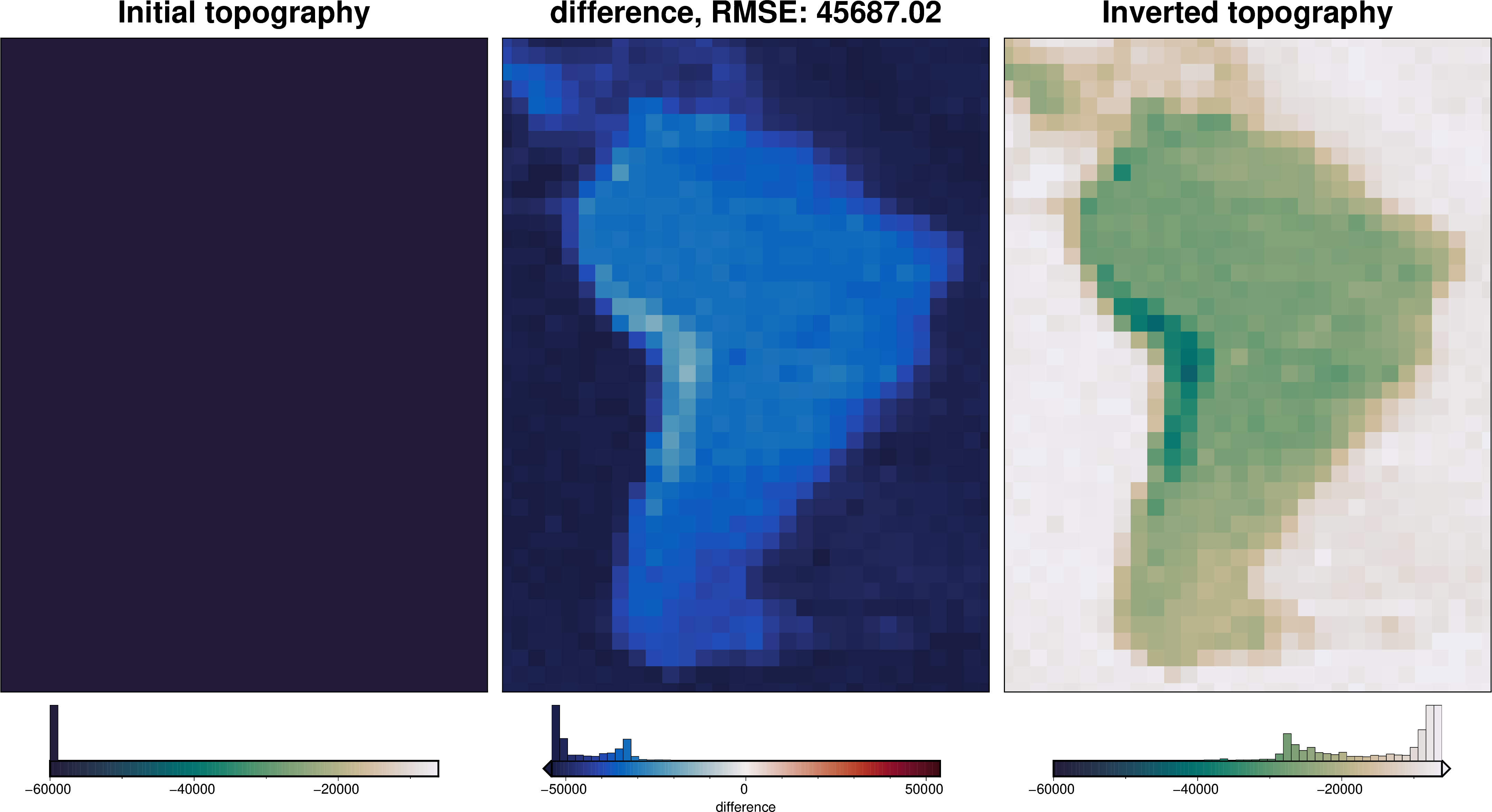
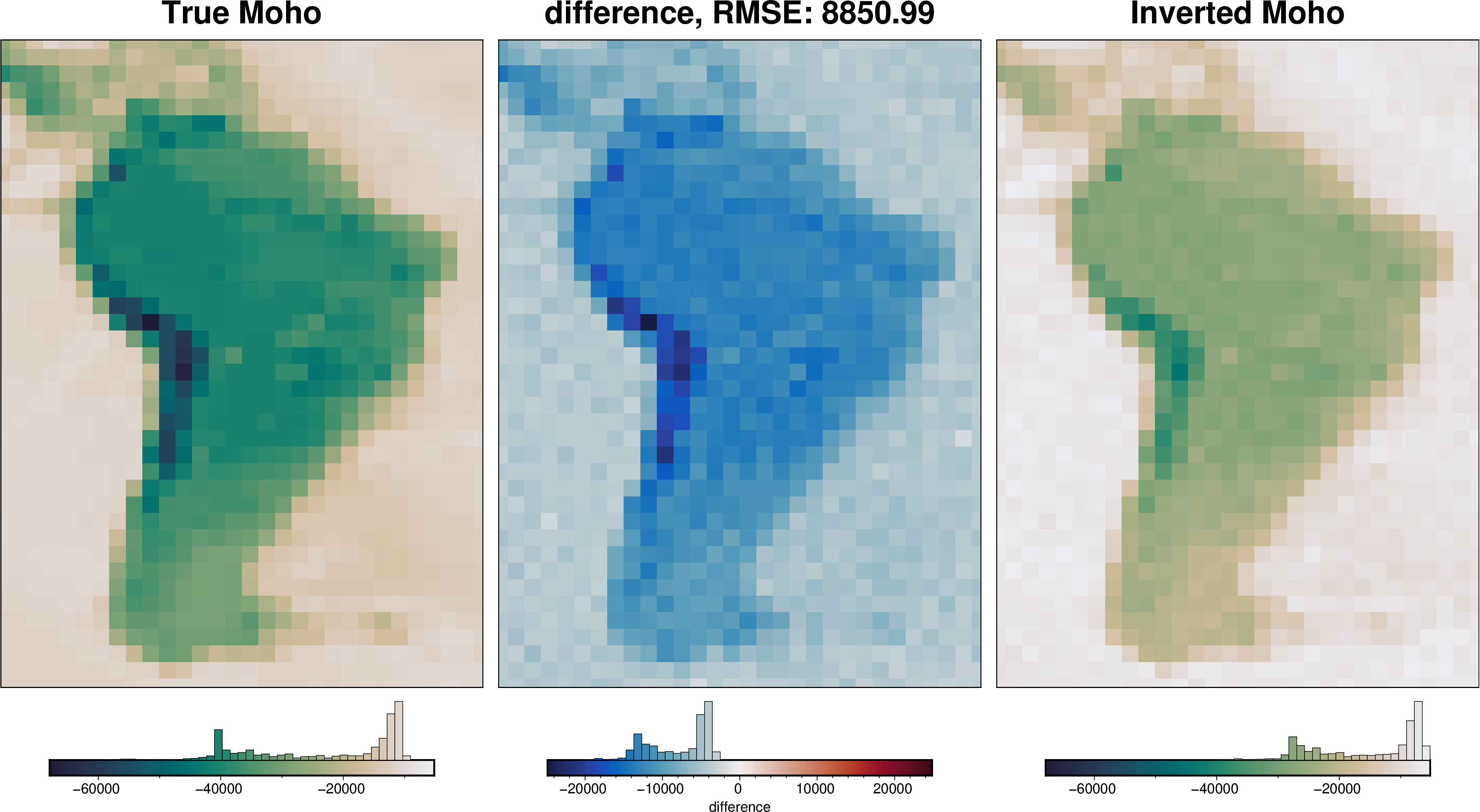
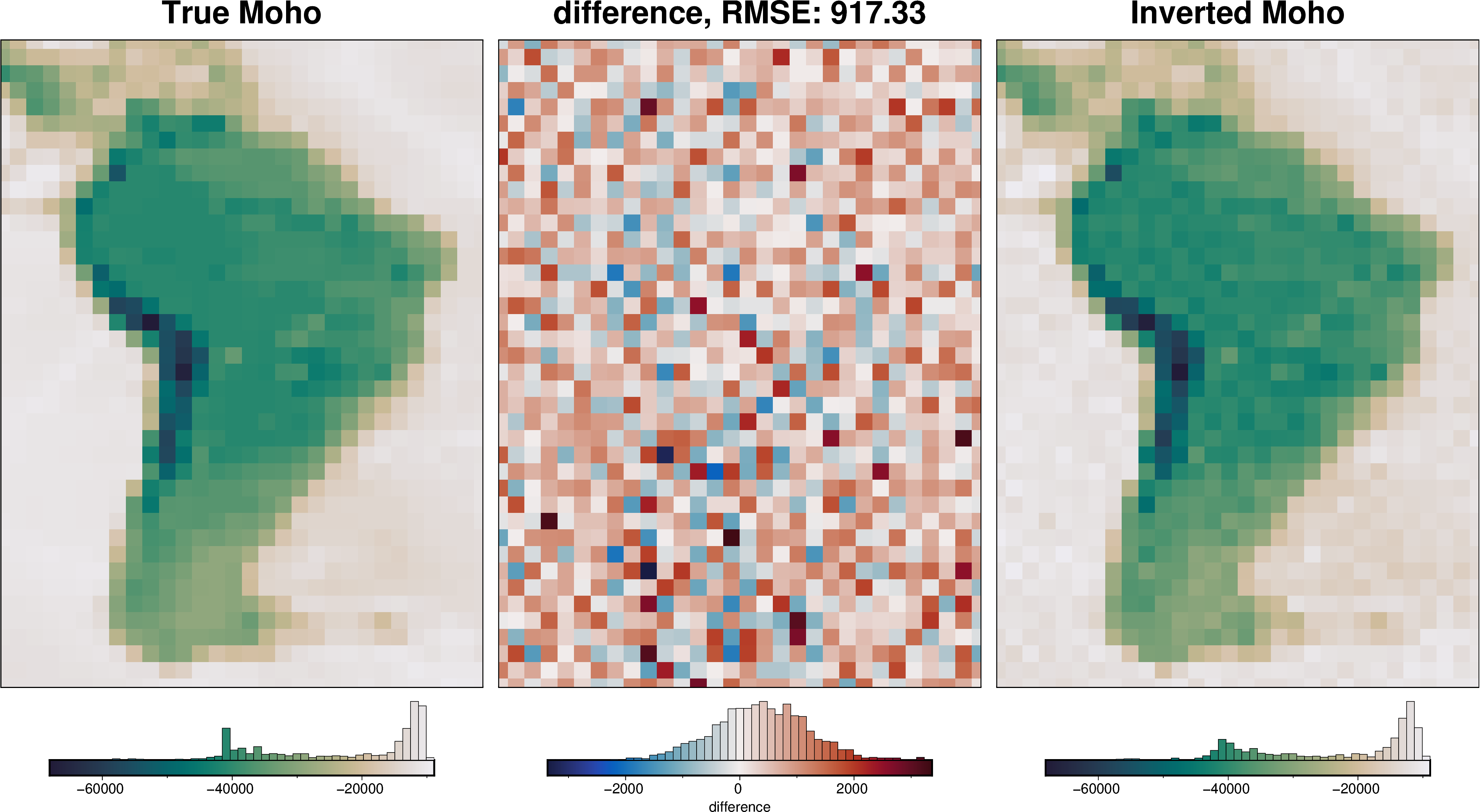
The below plot compares the true Moho model from CRUST1.0 with the inverted Moho. The middle and right subplots are equivalent to Figures 7 d and c in the paper, respectively. The max differences in our inversion were ~3.5 km, compared to the ~9 km in the study.
[27]:
_ = ptk.grid_compare(
    true_moho.upward,
    inv.model.topography,
    region=inv.model.inner_region,
    grid1_name="True Moho",
    grid2_name="Inverted Moho",
    hist=True,
    inset=False,
    title="difference",
    reverse_cpt=True,
    cmap="rain",
    coast=True,
    coast_version="gmt",
)
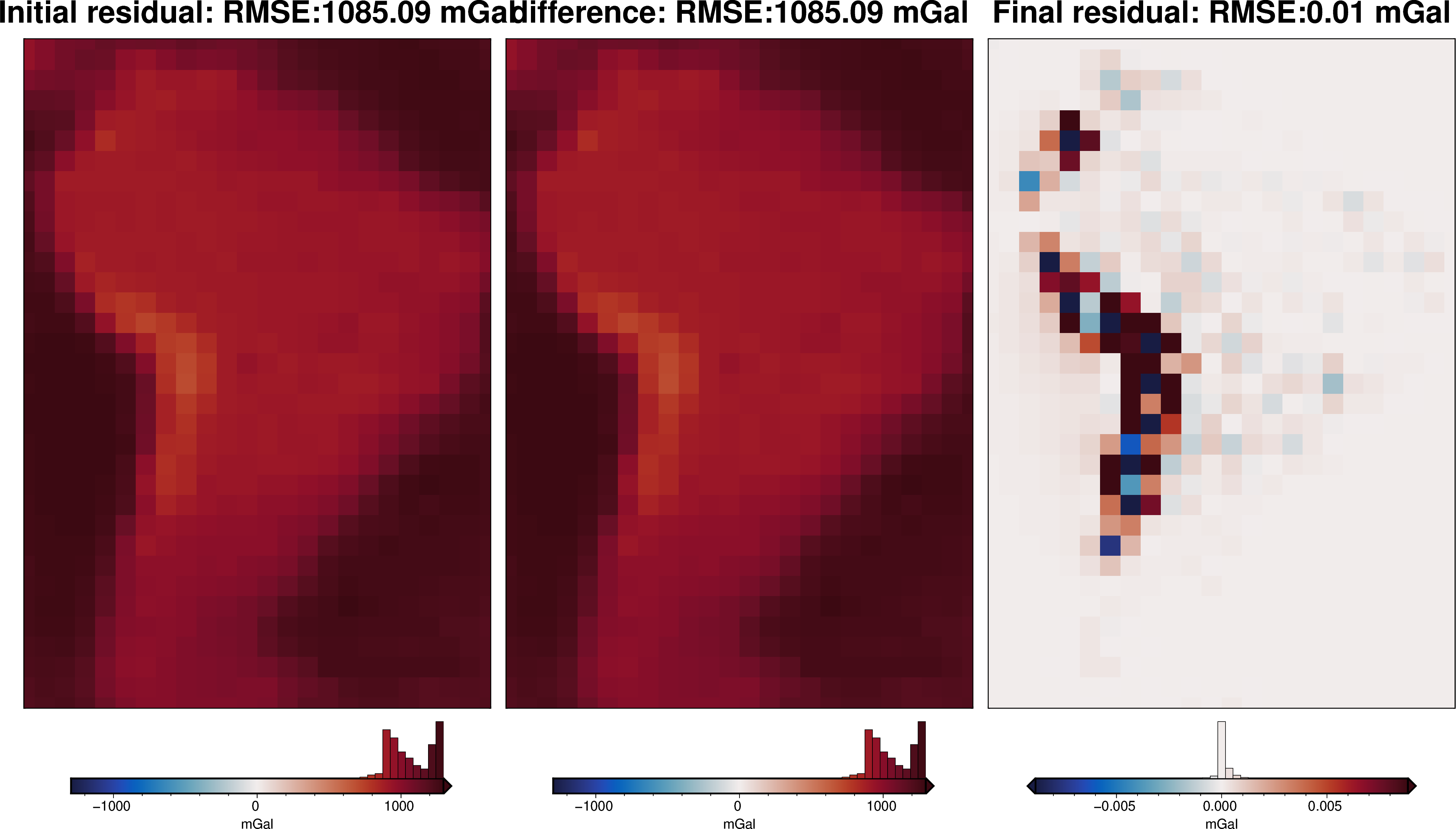
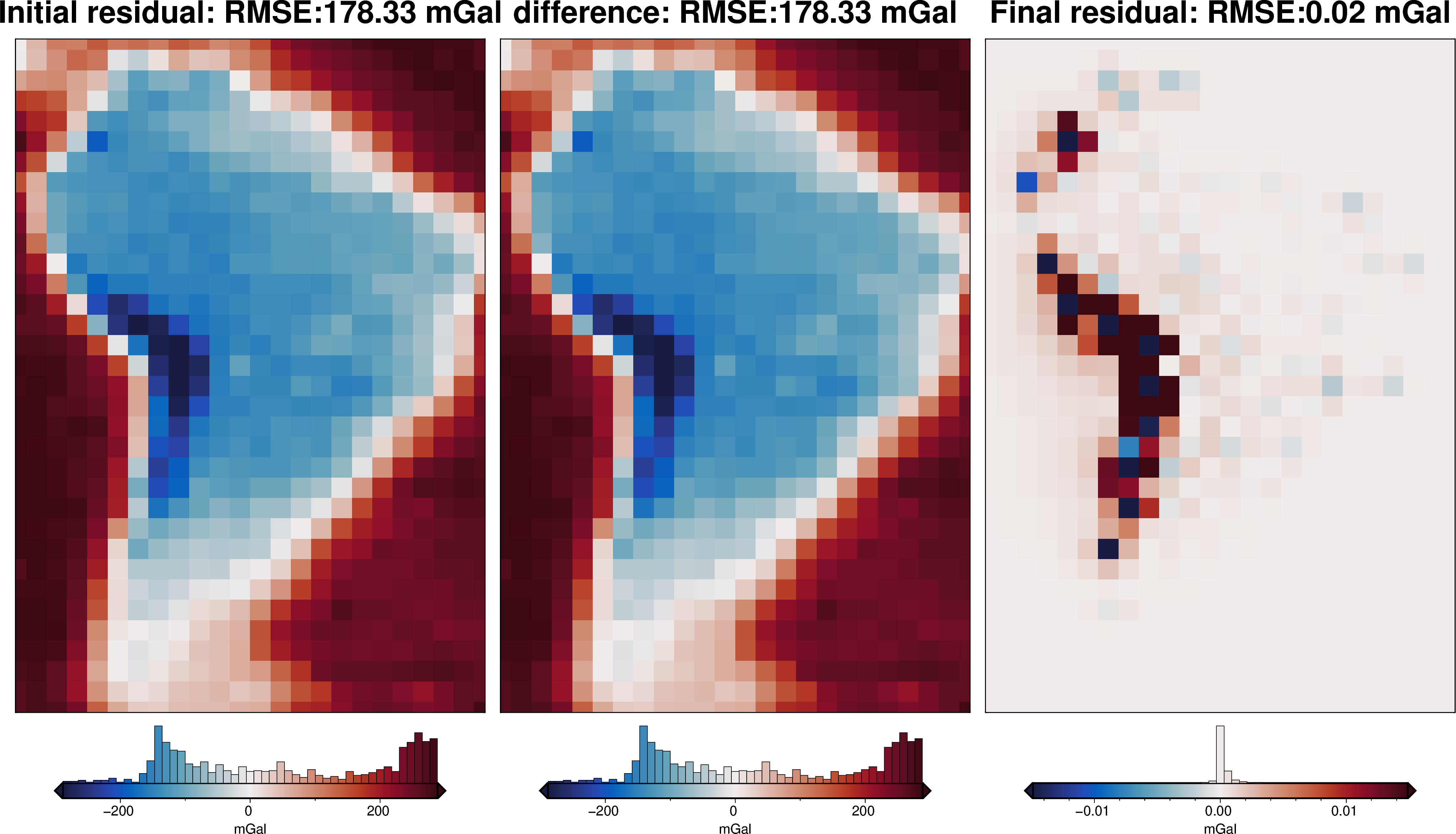
The below plot above compares gravity misfit before and after the inversion. The right subplot is equivalent to Figure 7g in the paper.
[28]:
inv.plot_inversion_results(
    iters_to_plot=2,
    fig_height=16,
    plot_grav_results=True,
    plot_topo_results=False,
    plot_iter_results=False,
)
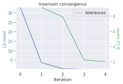
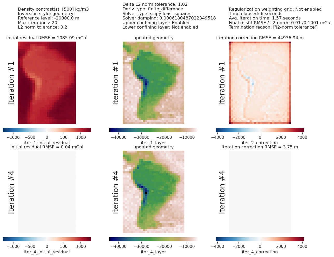
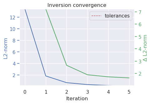
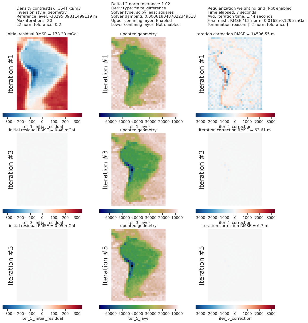
The below plot shows the iteration results of the inversion, and has all the parameter values and metadata at the top. From this, you can see the inversion terminated after 5 iterations due to the inversion reaching the set L2-norm tolerance.
[29]:
inv.plot_inversion_results(
    iters_to_plot=3,
    fig_height=16,
    plot_iter_results=True,
    plot_grav_results=False,
    plot_topo_results=False,
)
[30]:
# sample the inverted topography at the constraint points
constraint_points = invert4geom.sample_grids(
    constraint_points,
    inv.model.topography,
    "inverted_topography",
    coord_names=("longitude", "latitude"),
)

constraint_points["inversion_error"] = (
    constraint_points.upward - constraint_points.inverted_topography
)
rmse = invert4geom.rmse(constraint_points.inversion_error)
print(f"RMSE: {rmse:.2f} m")
RMSE: 800.10 m
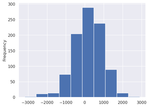
The below histogram is of the difference between the CRUST1.0 depths and the inverted depths at constraint points, equivalent to Figure 7f in the paper.
[31]:
constraint_points.inversion_error.plot.hist()
[31]:
<Axes: ylabel='Frequency'>
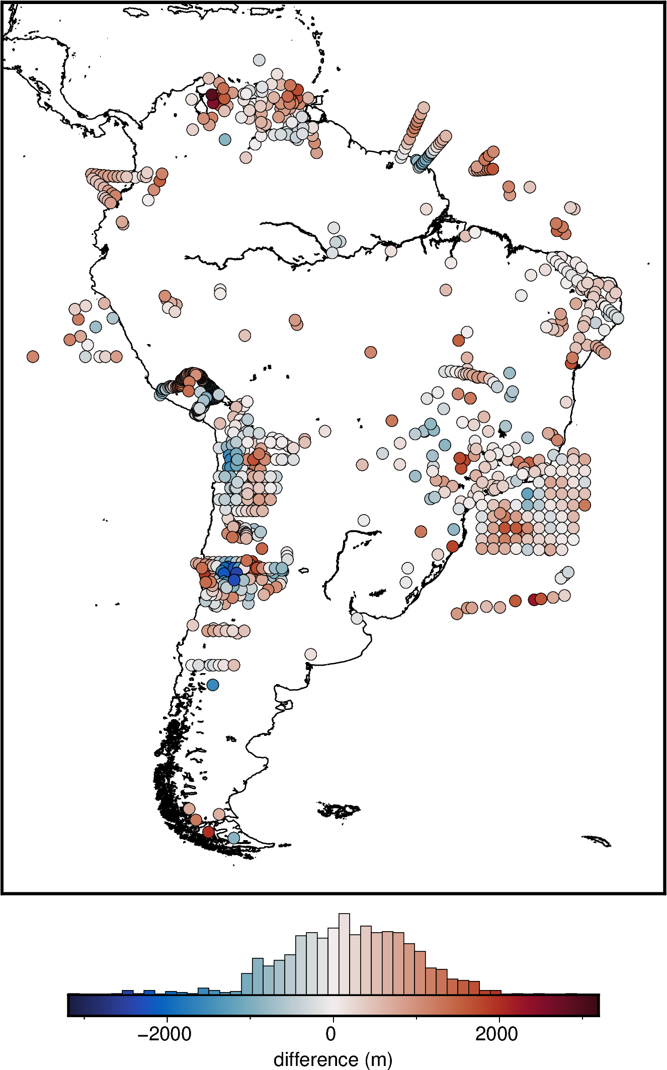
The below plot is equivalent to Figure 7 h in the paper.
[32]:
fig = ptk.basemap(
    region=inv.model.inner_region,
)

fig.coast(
    shorelines="0.5p,black",
)

fig.add_points(
    constraint_points.rename(columns={"longitude": "x", "latitude": "y"}),
    fill="inversion_error",
    pen=".2p,black",
    cmap="balance+h0",
    absolute=True,
    hist=True,
    cbar_label="difference (m)",
)

fig.show()
[ ]: