2. Simple inversionHere we will walkthrough a very simple gravity inversion using synthetic data. The goal of the inversion is to recover the geometry of a layer. In this case, the layer is simply the surface of the Earth, which is represented by the density contrast between air and rock.
2.1. Import packagesWe need to import the Invert4Geom package, as well as a few others.
/home/mdtanker/miniforge3/envs/invert4geom/lib/python3.12/site-packages/UQpy/__init__.py:6: UserWarning:

pkg_resources is deprecated as an API. See https://setuptools.pypa.io/en/latest/pkg_resources.html. The pkg_resources package is slated for removal as early as 2025-11-30. Refrain from using this package or pin to Setuptools<81.
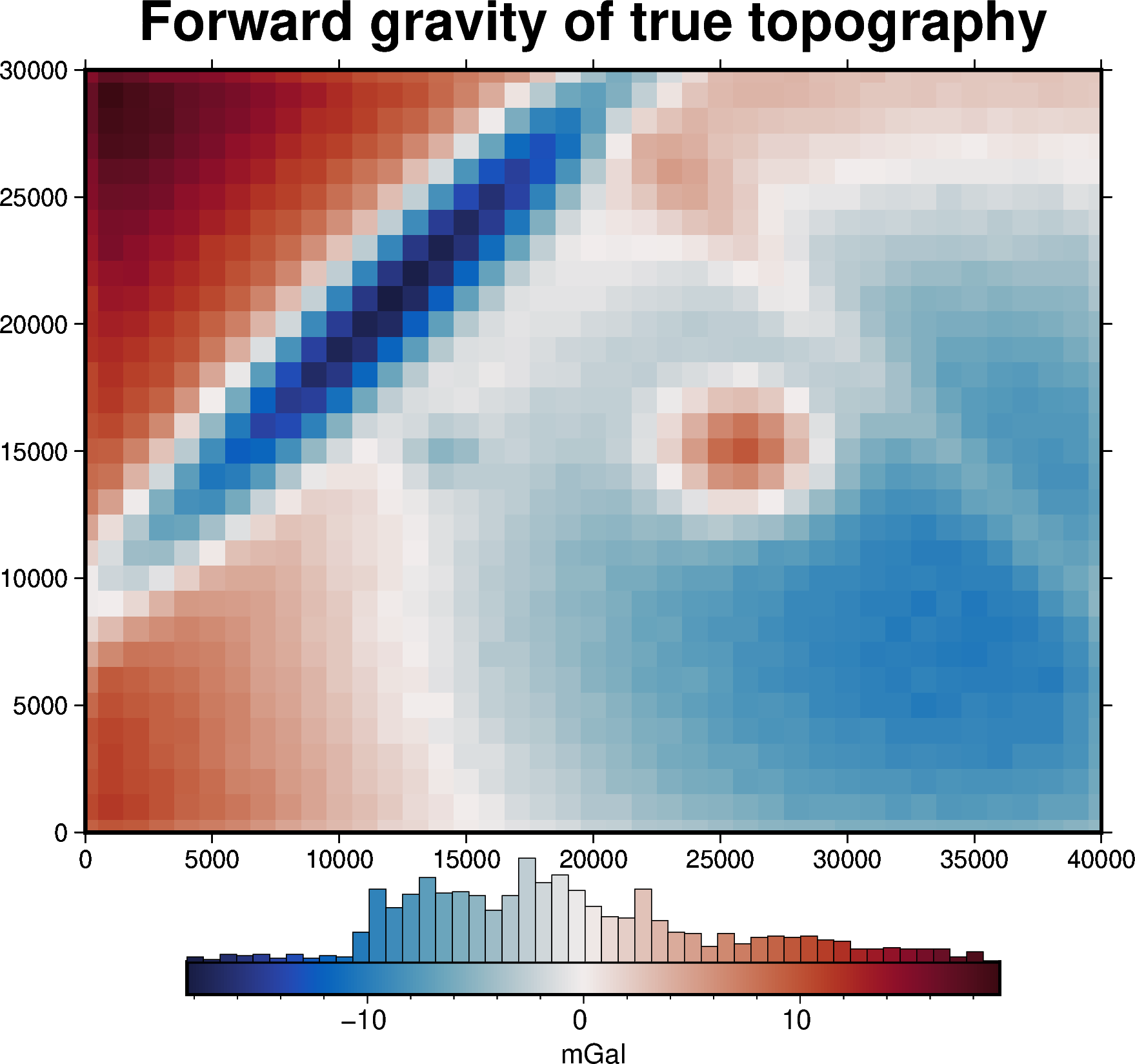
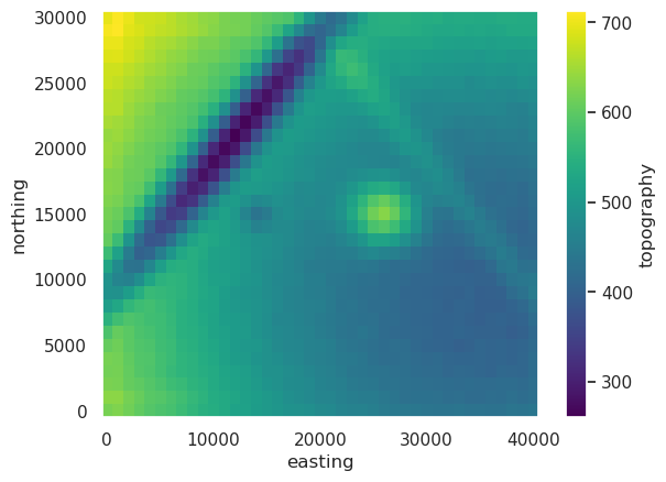
2.2. Create observed gravity dataTo run the inversion, we need to have observed gravity data. In this simple example, we will first create a synthetic topography grid, which represents the true Earth topography which we hope to recover during the inversion. The observed gravity will be the forward-calculated gravity effect of this topography.
Below we specify the spacing region zref density contrast
<xarray.Dataset> Size: 21kB
Dimensions:          (northing: 31, easting: 41)
Coordinates:
  * northing         (northing) float64 248B 0.0 1e+03 2e+03 ... 2.9e+04 3e+04
  * easting          (easting) float64 328B 0.0 1e+03 2e+03 ... 3.9e+04 4e+04
Data variables:
    upward           (northing, easting) float64 10kB 1e+03 1e+03 ... 1e+03
    gravity_anomaly  (northing, easting) float64 10kB 9.07 9.813 ... 2.527 2.473
2.3. Initialize the gravity dataThe observed gravity data needs to be in a gridded format, as an xarray Dataset with a variable gravity_anomaly upward easting northing longitude latitude
With this, we can use the create_data
region
spacing
buffer_width inner_region
inner_region
model_type
<xarray.Dataset> Size: 21kB
Dimensions: (northing: 31, easting: 41)
Coordinates:
* northing (northing) float64 248B 0.0 1e+03 2e+03 ... 2.9e+04 3e+04
* easting (easting) float64 328B 0.0 1e+03 2e+03 ... 3.9e+04 4e+04
Data variables:
upward (northing, easting) float64 10kB 1e+03 1e+03 ... 1e+03
gravity_anomaly (northing, easting) float64 10kB 9.07 9.813 ... 2.527 2.473
Attributes:
region: (0.0, 40000.0, 0.0, 30000.0)
spacing: 1000.0
buffer_width: 3000.0
inner_region: (3000.0, 37000.0, 3000.0, 27000.0)
dataset_type: data
model_type: prisms
coord_names: ('easting', 'northing')
Invert4Geom has an xarray dataset accessor inv
df
inner_df
inner
It also allows access to some methods:
forward_gravity
regional_separation
plot_observed
plot_anomalies
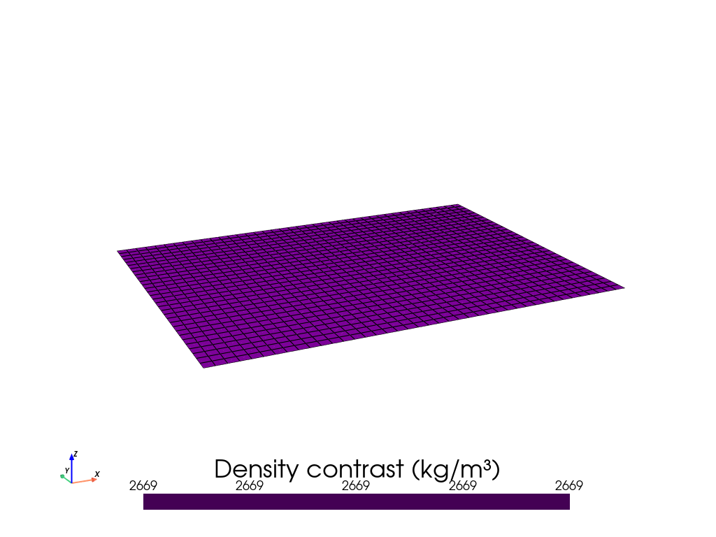
2.4. Create a starting topography gridHere we assume we know nothing about the topography, so we create a flat grid with a value of 500 m. Instead, you can use an existing topography model, as long as it’s an xarray Dataset with a variable upward easting northing longitude latitude
<xarray.Dataset> Size: 11kB
Dimensions: (northing: 31, easting: 41)
Coordinates:
* northing (northing) float64 248B 0.0 1e+03 2e+03 ... 2.8e+04 2.9e+04 3e+04
* easting (easting) float64 328B 0.0 1e+03 2e+03 ... 3.8e+04 3.9e+04 4e+04
Data variables:
upward (northing, easting) float64 10kB 500.0 500.0 500.0 ... 500.0 500.0
2.5. Create a Model objectNext, we can use the create_model the previous notebook create_model starting_topography topography mask upper_confining_layer lower_confining_layer
region
inner_region mask spacing
model_type
zref
density_contrast
<xarray.Dataset> Size: 92kB
Dimensions: (northing: 31, easting: 41)
Coordinates:
* northing (northing) float64 248B 0.0 1e+03 ... 2.9e+04 3e+04
* easting (easting) float64 328B 0.0 1e+03 ... 3.9e+04 4e+04
top (northing, easting) float64 10kB 500.0 ... 500.0
bottom (northing, easting) float64 10kB 500.0 ... 500.0
Data variables:
density (northing, easting) int64 10kB 2669 2669 ... 2669
thickness (northing, easting) float64 10kB 0.0 0.0 ... 0.0 0.0
starting_topography (northing, easting) float64 10kB 500.0 ... 500.0
topography (northing, easting) float64 10kB 500.0 ... 500.0
mask (northing, easting) float64 10kB 1.0 1.0 ... 1.0 1.0
upper_confining_layer (northing, easting) float64 10kB nan nan ... nan nan
lower_confining_layer (northing, easting) float64 10kB nan nan ... nan nan
Attributes:
zref: 500
density_contrast: 2669
region: (0.0, 40000.0, 0.0, 30000.0)
spacing: 1000.0
buffer_width: 0
inner_region: (0.0, 40000.0, 0.0, 30000.0)
dataset_type: model
model_type: prisms
coord_names: ('easting', 'northing') Dimensions: Coordinates: (4)
northing
(northing)
float64
0.0 1e+03 2e+03 ... 2.9e+04 3e+04
array([    0.,  1000.,  2000.,  3000.,  4000.,  5000.,  6000.,  7000.,  8000.,
        9000., 10000., 11000., 12000., 13000., 14000., 15000., 16000., 17000.,
       18000., 19000., 20000., 21000., 22000., 23000., 24000., 25000., 26000.,
       27000., 28000., 29000., 30000.])
easting
(easting)
float64
0.0 1e+03 2e+03 ... 3.9e+04 4e+04
array([    0.,  1000.,  2000.,  3000.,  4000.,  5000.,  6000.,  7000.,  8000.,
        9000., 10000., 11000., 12000., 13000., 14000., 15000., 16000., 17000.,
       18000., 19000., 20000., 21000., 22000., 23000., 24000., 25000., 26000.,
       27000., 28000., 29000., 30000., 31000., 32000., 33000., 34000., 35000.,
36000., 37000., 38000., 39000., 40000.]) top
(northing, easting)
float64
500.0 500.0 500.0 ... 500.0 500.0
array([[500., 500., 500., ..., 500., 500., 500.],
[500., 500., 500., ..., 500., 500., 500.],
[500., 500., 500., ..., 500., 500., 500.],
...,
[500., 500., 500., ..., 500., 500., 500.],
[500., 500., 500., ..., 500., 500., 500.],
[500., 500., 500., ..., 500., 500., 500.]], shape=(31, 41)) bottom
(northing, easting)
float64
500.0 500.0 500.0 ... 500.0 500.0
array([[500., 500., 500., ..., 500., 500., 500.],
[500., 500., 500., ..., 500., 500., 500.],
[500., 500., 500., ..., 500., 500., 500.],
...,
[500., 500., 500., ..., 500., 500., 500.],
[500., 500., 500., ..., 500., 500., 500.],
[500., 500., 500., ..., 500., 500., 500.]], shape=(31, 41)) Data variables: (7)
density
(northing, easting)
int64
2669 2669 2669 ... 2669 2669 2669
array([[2669, 2669, 2669, ..., 2669, 2669, 2669],
[2669, 2669, 2669, ..., 2669, 2669, 2669],
[2669, 2669, 2669, ..., 2669, 2669, 2669],
...,
[2669, 2669, 2669, ..., 2669, 2669, 2669],
[2669, 2669, 2669, ..., 2669, 2669, 2669],
[2669, 2669, 2669, ..., 2669, 2669, 2669]], shape=(31, 41)) thickness
(northing, easting)
float64
0.0 0.0 0.0 0.0 ... 0.0 0.0 0.0 0.0
array([[0., 0., 0., ..., 0., 0., 0.],
[0., 0., 0., ..., 0., 0., 0.],
[0., 0., 0., ..., 0., 0., 0.],
...,
[0., 0., 0., ..., 0., 0., 0.],
[0., 0., 0., ..., 0., 0., 0.],
[0., 0., 0., ..., 0., 0., 0.]], shape=(31, 41)) starting_topography
(northing, easting)
float64
500.0 500.0 500.0 ... 500.0 500.0
array([[500., 500., 500., ..., 500., 500., 500.],
[500., 500., 500., ..., 500., 500., 500.],
[500., 500., 500., ..., 500., 500., 500.],
...,
[500., 500., 500., ..., 500., 500., 500.],
[500., 500., 500., ..., 500., 500., 500.],
[500., 500., 500., ..., 500., 500., 500.]], shape=(31, 41)) topography
(northing, easting)
float64
500.0 500.0 500.0 ... 500.0 500.0
array([[500., 500., 500., ..., 500., 500., 500.],
[500., 500., 500., ..., 500., 500., 500.],
[500., 500., 500., ..., 500., 500., 500.],
...,
[500., 500., 500., ..., 500., 500., 500.],
[500., 500., 500., ..., 500., 500., 500.],
[500., 500., 500., ..., 500., 500., 500.]], shape=(31, 41)) mask
(northing, easting)
float64
1.0 1.0 1.0 1.0 ... 1.0 1.0 1.0 1.0
array([[1., 1., 1., ..., 1., 1., 1.],
[1., 1., 1., ..., 1., 1., 1.],
[1., 1., 1., ..., 1., 1., 1.],
...,
[1., 1., 1., ..., 1., 1., 1.],
[1., 1., 1., ..., 1., 1., 1.],
[1., 1., 1., ..., 1., 1., 1.]], shape=(31, 41)) upper_confining_layer
(northing, easting)
float64
nan nan nan nan ... nan nan nan nan
array([[nan, nan, nan, ..., nan, nan, nan],
[nan, nan, nan, ..., nan, nan, nan],
[nan, nan, nan, ..., nan, nan, nan],
...,
[nan, nan, nan, ..., nan, nan, nan],
[nan, nan, nan, ..., nan, nan, nan],
[nan, nan, nan, ..., nan, nan, nan]], shape=(31, 41)) lower_confining_layer
(northing, easting)
float64
nan nan nan nan ... nan nan nan nan
array([[nan, nan, nan, ..., nan, nan, nan],
[nan, nan, nan, ..., nan, nan, nan],
[nan, nan, nan, ..., nan, nan, nan],
...,
[nan, nan, nan, ..., nan, nan, nan],
[nan, nan, nan, ..., nan, nan, nan],
[nan, nan, nan, ..., nan, nan, nan]], shape=(31, 41)) Attributes: (9)
zref : 500 density_contrast : 2669 region : (0.0, 40000.0, 0.0, 30000.0) spacing : 1000.0 buffer_width : 0 inner_region : (0.0, 40000.0, 0.0, 30000.0) dataset_type : model model_type : prisms coord_names : ('easting', 'northing')
The same Invert4Geom xarray dataset accessor inv
df
inner_df
inner
masked mask
masked_df
It also allows access to some methods:
2.6. Gravity misfitNow we need to use this starting prism model to calculate the gravity misfit, which is the difference between the observed gravity and the gravity effect of this starting prism model. If this case, the starting model is flat, so it has no gravity effect.
To calculate the forward gravity effect of the starting model, use the inv dataset accessor forward_gravity
<xarray.Dataset> Size: 31kB
Dimensions: (northing: 31, easting: 41)
Coordinates:
* northing (northing) float64 248B 0.0 1e+03 2e+03 ... 2.9e+04 3e+04
* easting (easting) float64 328B 0.0 1e+03 2e+03 ... 3.9e+04 4e+04
Data variables:
upward (northing, easting) float64 10kB 1e+03 1e+03 ... 1e+03
gravity_anomaly (northing, easting) float64 10kB 9.07 9.813 ... 2.527 2.473
forward_gravity (northing, easting) float64 10kB -0.0 -0.0 ... -0.0 -0.0
Attributes:
region: (0.0, 40000.0, 0.0, 30000.0)
spacing: 1000.0
buffer_width: 3000.0
inner_region: (3000.0, 37000.0, 3000.0, 27000.0)
dataset_type: data
model_type: prisms
coord_names: ('easting', 'northing') Dimensions: Coordinates: (2)
Data variables: (3)
upward
(northing, easting)
float64
1e+03 1e+03 1e+03 ... 1e+03 1e+03
array([[1000., 1000., 1000., ..., 1000., 1000., 1000.],
       [1000., 1000., 1000., ..., 1000., 1000., 1000.],
       [1000., 1000., 1000., ..., 1000., 1000., 1000.],
       ...,
       [1000., 1000., 1000., ..., 1000., 1000., 1000.],
       [1000., 1000., 1000., ..., 1000., 1000., 1000.],
       [1000., 1000., 1000., ..., 1000., 1000., 1000.]], shape=(31, 41))
gravity_anomaly
(northing, easting)
float64
9.07 9.813 9.473 ... 2.527 2.473
array([[ 9.06960365,  9.81322676,  9.47333418, ..., -5.61435085,
        -5.19228994, -4.7861235 ],
       [10.52345435, 11.524123  , 10.87441465, ..., -6.93271041,
        -6.92947076, -5.83707679],
       [10.11443708, 11.03336324, 10.46857842, ..., -7.91375604,
        -7.48700667, -6.24682833],
       ...,
       [16.77703767, 18.74270979, 18.3048348 , ...,  1.47098018,
         1.53072568,  1.60815283],
       [16.78520431, 19.22032586, 18.33502618, ...,  2.63546487,
         2.45011455,  2.35237476],
       [15.10949873, 17.11895624, 16.78130574, ...,  2.78791601,
2.52700439, 2.47270992]], shape=(31, 41)) forward_gravity
(northing, easting)
float64
-0.0 -0.0 -0.0 ... -0.0 -0.0 -0.0
array([[-0., -0., -0., ..., -0., -0., -0.],
[-0., -0., -0., ..., -0., -0., -0.],
[-0., -0., -0., ..., -0., -0., -0.],
...,
[-0., -0., -0., ..., -0., -0., -0.],
[-0., -0., -0., ..., -0., -0., -0.],
[-0., -0., -0., ..., -0., -0., -0.]], shape=(31, 41)) Attributes: (7)
region : (0.0, 40000.0, 0.0, 30000.0) spacing : 1000.0 buffer_width : 3000.0 inner_region : (3000.0, 37000.0, 3000.0, 27000.0) dataset_type : data model_type : prisms coord_names : ('easting', 'northing')
In many cases, we want to remove a regional signal from the misfit to isolate the residual signal. In this simple case, we assume there is no regional component to the misfit and set it to 0. The inv dataset accessor regional_separation forward_gravity gravity_anomaly misfit reg misfit res
<xarray.Dataset> Size: 102kB
Dimensions: (northing: 31, easting: 41)
Coordinates:
* northing (northing) float64 248B 0.0 1e+03 ... 3e+04
* easting (easting) float64 328B 0.0 1e+03 ... 3.9e+04 4e+04
Data variables:
upward (northing, easting) float64 10kB 1e+03 ... 1e+03
gravity_anomaly (northing, easting) float64 10kB 9.07 ... 2.473
forward_gravity (northing, easting) float64 10kB -0.0 ... -0.0
misfit (northing, easting) float64 10kB 9.07 ... 2.473
reg (northing, easting) float64 10kB 0.0 0.0 ... 0.0
res (northing, easting) float64 10kB 9.07 ... 2.473
starting_forward_gravity (northing, easting) float64 10kB -0.0 ... -0.0
starting_misfit (northing, easting) float64 10kB 9.07 ... 2.473
starting_reg (northing, easting) float64 10kB 0.0 0.0 ... 0.0
starting_res (northing, easting) float64 10kB 9.07 ... 2.473
Attributes:
region: (0.0, 40000.0, 0.0, 30000.0)
spacing: 1000.0
buffer_width: 3000.0
inner_region: (3000.0, 37000.0, 3000.0, 27000.0)
dataset_type: data
model_type: prisms
coord_names: ('easting', 'northing') Dimensions: Coordinates: (2)
Data variables: (10)
upward
(northing, easting)
float64
1e+03 1e+03 1e+03 ... 1e+03 1e+03
array([[1000., 1000., 1000., ..., 1000., 1000., 1000.],
[1000., 1000., 1000., ..., 1000., 1000., 1000.],
[1000., 1000., 1000., ..., 1000., 1000., 1000.],
...,
[1000., 1000., 1000., ..., 1000., 1000., 1000.],
[1000., 1000., 1000., ..., 1000., 1000., 1000.],
[1000., 1000., 1000., ..., 1000., 1000., 1000.]], shape=(31, 41)) gravity_anomaly
(northing, easting)
float64
9.07 9.813 9.473 ... 2.527 2.473
array([[ 9.06960365, 9.81322676, 9.47333418, ..., -5.61435085,
-5.19228994, -4.7861235 ],
[10.52345435, 11.524123 , 10.87441465, ..., -6.93271041,
-6.92947076, -5.83707679],
[10.11443708, 11.03336324, 10.46857842, ..., -7.91375604,
-7.48700667, -6.24682833],
...,
[16.77703767, 18.74270979, 18.3048348 , ..., 1.47098018,
1.53072568, 1.60815283],
[16.78520431, 19.22032586, 18.33502618, ..., 2.63546487,
2.45011455, 2.35237476],
[15.10949873, 17.11895624, 16.78130574, ..., 2.78791601,
2.52700439, 2.47270992]], shape=(31, 41)) forward_gravity
(northing, easting)
float64
-0.0 -0.0 -0.0 ... -0.0 -0.0 -0.0
array([[-0., -0., -0., ..., -0., -0., -0.],
[-0., -0., -0., ..., -0., -0., -0.],
[-0., -0., -0., ..., -0., -0., -0.],
...,
[-0., -0., -0., ..., -0., -0., -0.],
[-0., -0., -0., ..., -0., -0., -0.],
[-0., -0., -0., ..., -0., -0., -0.]], shape=(31, 41)) misfit
(northing, easting)
float64
9.07 9.813 9.473 ... 2.527 2.473
array([[ 9.06960365, 9.81322676, 9.47333418, ..., -5.61435085,
-5.19228994, -4.7861235 ],
[10.52345435, 11.524123 , 10.87441465, ..., -6.93271041,
-6.92947076, -5.83707679],
[10.11443708, 11.03336324, 10.46857842, ..., -7.91375604,
-7.48700667, -6.24682833],
...,
[16.77703767, 18.74270979, 18.3048348 , ..., 1.47098018,
1.53072568, 1.60815283],
[16.78520431, 19.22032586, 18.33502618, ..., 2.63546487,
2.45011455, 2.35237476],
[15.10949873, 17.11895624, 16.78130574, ..., 2.78791601,
2.52700439, 2.47270992]], shape=(31, 41)) reg
(northing, easting)
float64
0.0 0.0 0.0 0.0 ... 0.0 0.0 0.0 0.0
array([[0., 0., 0., ..., 0., 0., 0.],
[0., 0., 0., ..., 0., 0., 0.],
[0., 0., 0., ..., 0., 0., 0.],
...,
[0., 0., 0., ..., 0., 0., 0.],
[0., 0., 0., ..., 0., 0., 0.],
[0., 0., 0., ..., 0., 0., 0.]], shape=(31, 41)) res
(northing, easting)
float64
9.07 9.813 9.473 ... 2.527 2.473
array([[ 9.06960365, 9.81322676, 9.47333418, ..., -5.61435085,
-5.19228994, -4.7861235 ],
[10.52345435, 11.524123 , 10.87441465, ..., -6.93271041,
-6.92947076, -5.83707679],
[10.11443708, 11.03336324, 10.46857842, ..., -7.91375604,
-7.48700667, -6.24682833],
...,
[16.77703767, 18.74270979, 18.3048348 , ..., 1.47098018,
1.53072568, 1.60815283],
[16.78520431, 19.22032586, 18.33502618, ..., 2.63546487,
2.45011455, 2.35237476],
[15.10949873, 17.11895624, 16.78130574, ..., 2.78791601,
2.52700439, 2.47270992]], shape=(31, 41)) starting_forward_gravity
(northing, easting)
float64
-0.0 -0.0 -0.0 ... -0.0 -0.0 -0.0
array([[-0., -0., -0., ..., -0., -0., -0.],
[-0., -0., -0., ..., -0., -0., -0.],
[-0., -0., -0., ..., -0., -0., -0.],
...,
[-0., -0., -0., ..., -0., -0., -0.],
[-0., -0., -0., ..., -0., -0., -0.],
[-0., -0., -0., ..., -0., -0., -0.]], shape=(31, 41)) starting_misfit
(northing, easting)
float64
9.07 9.813 9.473 ... 2.527 2.473
array([[ 9.06960365, 9.81322676, 9.47333418, ..., -5.61435085,
-5.19228994, -4.7861235 ],
[10.52345435, 11.524123 , 10.87441465, ..., -6.93271041,
-6.92947076, -5.83707679],
[10.11443708, 11.03336324, 10.46857842, ..., -7.91375604,
-7.48700667, -6.24682833],
...,
[16.77703767, 18.74270979, 18.3048348 , ..., 1.47098018,
1.53072568, 1.60815283],
[16.78520431, 19.22032586, 18.33502618, ..., 2.63546487,
2.45011455, 2.35237476],
[15.10949873, 17.11895624, 16.78130574, ..., 2.78791601,
2.52700439, 2.47270992]], shape=(31, 41)) starting_reg
(northing, easting)
float64
0.0 0.0 0.0 0.0 ... 0.0 0.0 0.0 0.0
array([[0., 0., 0., ..., 0., 0., 0.],
[0., 0., 0., ..., 0., 0., 0.],
[0., 0., 0., ..., 0., 0., 0.],
...,
[0., 0., 0., ..., 0., 0., 0.],
[0., 0., 0., ..., 0., 0., 0.],
[0., 0., 0., ..., 0., 0., 0.]], shape=(31, 41)) starting_res
(northing, easting)
float64
9.07 9.813 9.473 ... 2.527 2.473
array([[ 9.06960365, 9.81322676, 9.47333418, ..., -5.61435085,
-5.19228994, -4.7861235 ],
[10.52345435, 11.524123 , 10.87441465, ..., -6.93271041,
-6.92947076, -5.83707679],
[10.11443708, 11.03336324, 10.46857842, ..., -7.91375604,
-7.48700667, -6.24682833],
...,
[16.77703767, 18.74270979, 18.3048348 , ..., 1.47098018,
1.53072568, 1.60815283],
[16.78520431, 19.22032586, 18.33502618, ..., 2.63546487,
2.45011455, 2.35237476],
[15.10949873, 17.11895624, 16.78130574, ..., 2.78791601,
2.52700439, 2.47270992]], shape=(31, 41)) Attributes: (7)
region : (0.0, 40000.0, 0.0, 30000.0) spacing : 1000.0 buffer_width : 3000.0 inner_region : (3000.0, 37000.0, 3000.0, 27000.0) dataset_type : data model_type : prisms coord_names : ('easting', 'northing')
We can plot all these anomalies with the accessor function plot_anomalies
makecpt [ERROR]: Option T: min >= max
2.7. Initialize the Inversion classThe class Inversion data model
max_iterations
l2_norm_tolerance
delta_l2_norm_tolerance
solver_damping
apply_weighting_grid weighting_grid
During the inversion, instance attributes will be added such as the current iteration, the L2-norm and the computation time. The attributes data model
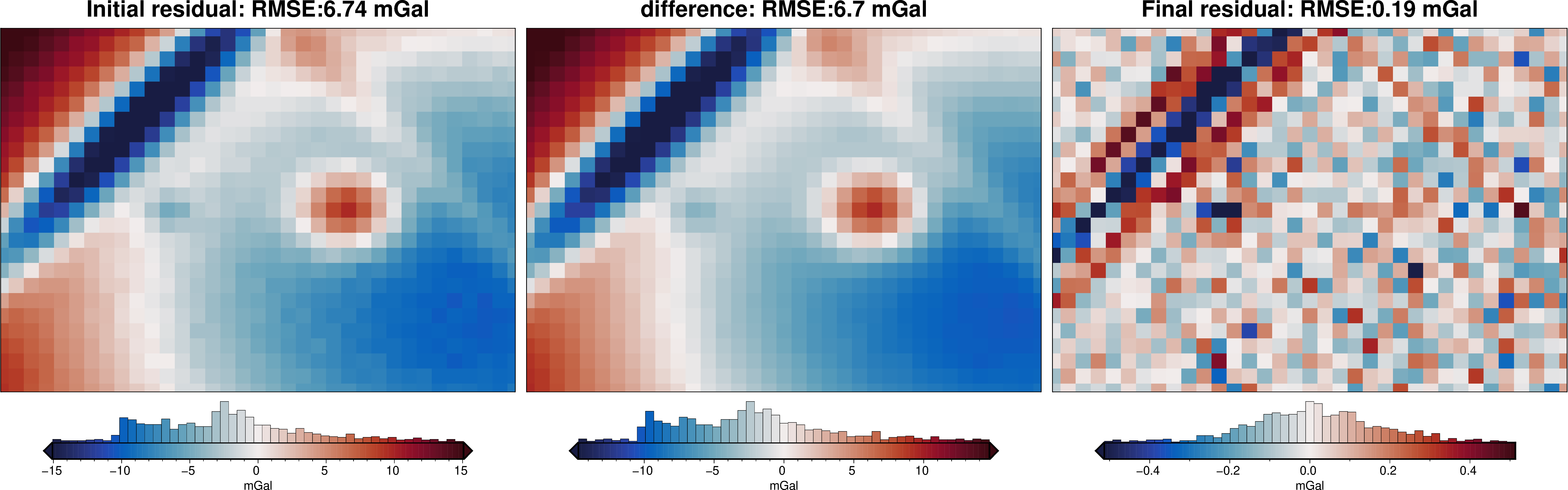
2.8. Perform inversionNow that we have the Inversion object which holds the starting model and residual gravity misfit data we can start the inversion. As the inversion progresses, the attributes inv.data inv.model
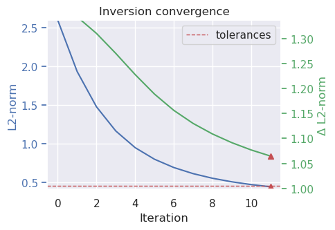
The above plot shows how the l2-norm and delta l2-norm have been reduced during the inversion. The red line at the bottom marks the set tolerances for each of these. This show that the inversion terminated at the 12 inversion since the l2-norm was lower than the set l2-norm tolerance.
We can access the statistics of the inversion results with the attribute stats_df
iteration
rmse
l2_norm
delta_l2_norm
iter_time_sec
0
0.0
6.743327
2.596792
inf
NaN
1
1.0
3.737865
1.933356
1.343153
0.685592
2
2.0
2.178281
1.475900
1.309950
0.124484
3
3.0
1.350640
1.162170
1.269952
0.126689
4
4.0
0.896104
0.946628
1.227695
0.127047
5
5.0
0.634186
0.796358
1.188697
0.132842
6
6.0
0.474482
0.688827
1.156108
0.142375
7
7.0
0.371599
0.609589
1.129985
0.153705
8
8.0
0.302185
0.549713
1.108922
0.156976
9
9.0
0.253624
0.503611
1.091543
0.150536
10
10.0
0.218663
0.467615
1.076979
0.161218
11
11.0
0.192876
0.439176
1.064753
0.161538
We can see why the inversion terminated with termination_reason
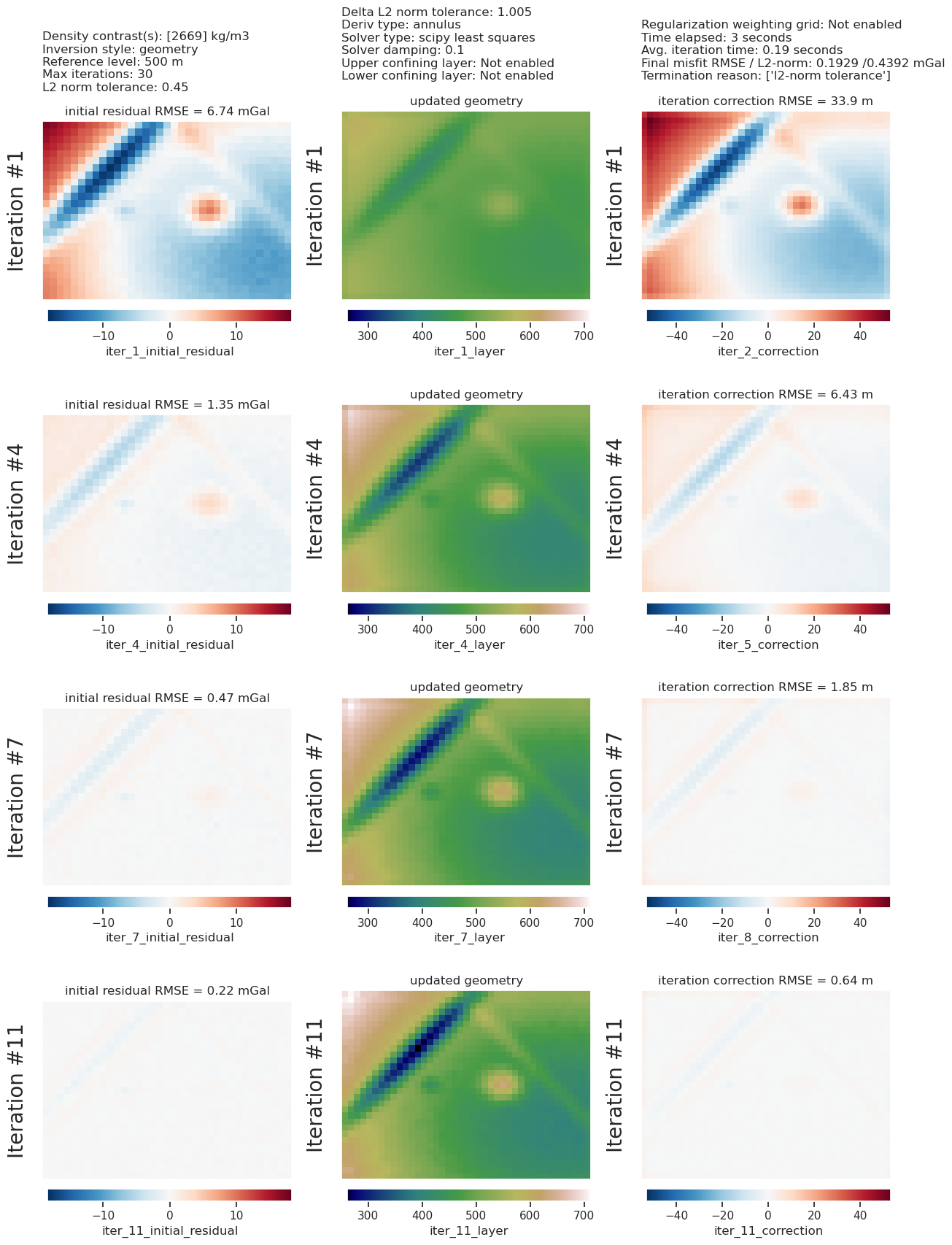
We can see the gravity data for each iteration:
<xarray.Dataset> Size: 214kB
Dimensions: (northing: 31, easting: 41)
Coordinates:
* northing (northing) float64 248B 0.0 1e+03 ... 3e+04
* easting (easting) float64 328B 0.0 1e+03 ... 3.9e+04 4e+04
Data variables: (12/21)
upward (northing, easting) float64 10kB 1e+03 ... 1e+03
gravity_anomaly (northing, easting) float64 10kB 9.07 ... 2.473
forward_gravity (northing, easting) float64 10kB 8.229 ... 2.094
misfit (northing, easting) float64 10kB 9.07 ... 2.473
reg (northing, easting) float64 10kB 0.0 0.0 ... 0.0
res (northing, easting) float64 10kB 0.841 ... 0.379
... ...
iter_6_initial_residual (northing, easting) float64 10kB 2.435 ... 0.8778
iter_7_initial_residual (northing, easting) float64 10kB 1.982 ... 0.7426
iter_8_initial_residual (northing, easting) float64 10kB 1.635 ... 0.6361
iter_9_initial_residual (northing, easting) float64 10kB 1.365 ... 0.551
iter_10_initial_residual (northing, easting) float64 10kB 1.152 ... 0.4822
iter_11_initial_residual (northing, easting) float64 10kB 0.9804 ... 0.4258
Attributes:
region: (0.0, 40000.0, 0.0, 30000.0)
spacing: 1000.0
buffer_width: 3000.0
inner_region: (3000.0, 37000.0, 3000.0, 27000.0)
dataset_type: data
model_type: prisms
coord_names: ('easting', 'northing') Dimensions: Coordinates: (2)
Data variables: (21)
upward
(northing, easting)
float64
1e+03 1e+03 1e+03 ... 1e+03 1e+03
array([[1000., 1000., 1000., ..., 1000., 1000., 1000.],
[1000., 1000., 1000., ..., 1000., 1000., 1000.],
[1000., 1000., 1000., ..., 1000., 1000., 1000.],
...,
[1000., 1000., 1000., ..., 1000., 1000., 1000.],
[1000., 1000., 1000., ..., 1000., 1000., 1000.],
[1000., 1000., 1000., ..., 1000., 1000., 1000.]], shape=(31, 41)) gravity_anomaly
(northing, easting)
float64
9.07 9.813 9.473 ... 2.527 2.473
array([[ 9.06960365, 9.81322676, 9.47333418, ..., -5.61435085,
-5.19228994, -4.7861235 ],
[10.52345435, 11.524123 , 10.87441465, ..., -6.93271041,
-6.92947076, -5.83707679],
[10.11443708, 11.03336324, 10.46857842, ..., -7.91375604,
-7.48700667, -6.24682833],
...,
[16.77703767, 18.74270979, 18.3048348 , ..., 1.47098018,
1.53072568, 1.60815283],
[16.78520431, 19.22032586, 18.33502618, ..., 2.63546487,
2.45011455, 2.35237476],
[15.10949873, 17.11895624, 16.78130574, ..., 2.78791601,
2.52700439, 2.47270992]], shape=(31, 41)) forward_gravity
(northing, easting)
float64
8.229 9.658 9.184 ... 2.506 2.094
array([[ 8.22864871, 9.65847467, 9.18402394, ..., -5.45468991,
-5.1976233 , -4.23112993],
[10.1801681 , 11.74440933, 10.99796924, ..., -7.17434642,
-6.94454687, -5.58281297],
[ 9.81447291, 11.28599088, 10.60967554, ..., -7.97354248,
-7.66214653, -6.06994138],
...,
[16.35623088, 18.97317291, 18.38478338, ..., 1.54241789,
1.57122506, 1.43252836],
[16.57327667, 19.52969188, 18.65664254, ..., 2.60003366,
2.57927916, 2.21387254],
[13.97821308, 16.8268703 , 16.27715346, ..., 2.63218901,
2.5057452 , 2.09370954]], shape=(31, 41)) misfit
(northing, easting)
float64
9.07 9.813 9.473 ... 2.527 2.473
array([[ 9.06960365, 9.81322676, 9.47333418, ..., -5.61435085,
-5.19228994, -4.7861235 ],
[10.52345435, 11.524123 , 10.87441465, ..., -6.93271041,
-6.92947076, -5.83707679],
[10.11443708, 11.03336324, 10.46857842, ..., -7.91375604,
-7.48700667, -6.24682833],
...,
[16.77703767, 18.74270979, 18.3048348 , ..., 1.47098018,
1.53072568, 1.60815283],
[16.78520431, 19.22032586, 18.33502618, ..., 2.63546487,
2.45011455, 2.35237476],
[15.10949873, 17.11895624, 16.78130574, ..., 2.78791601,
2.52700439, 2.47270992]], shape=(31, 41)) reg
(northing, easting)
float64
0.0 0.0 0.0 0.0 ... 0.0 0.0 0.0 0.0
array([[0., 0., 0., ..., 0., 0., 0.],
[0., 0., 0., ..., 0., 0., 0.],
[0., 0., 0., ..., 0., 0., 0.],
...,
[0., 0., 0., ..., 0., 0., 0.],
[0., 0., 0., ..., 0., 0., 0.],
[0., 0., 0., ..., 0., 0., 0.]], shape=(31, 41)) res
(northing, easting)
float64
0.841 0.1548 ... 0.02126 0.379
array([[ 0.84095494, 0.15475209, 0.28931024, ..., -0.15966094,
0.00533336, -0.55499357],
[ 0.34328625, -0.22028633, -0.12355459, ..., 0.24163601,
0.01507611, -0.25426383],
[ 0.29996418, -0.25262764, -0.14109711, ..., 0.05978644,
0.17513986, -0.17688695],
...,
[ 0.4208068 , -0.23046312, -0.07994859, ..., -0.07143771,
-0.04049938, 0.17562448],
[ 0.21192765, -0.30936602, -0.32161636, ..., 0.03543121,
-0.12916461, 0.13850222],
[ 1.13128565, 0.29208593, 0.50415229, ..., 0.155727 ,
0.02125919, 0.37900038]], shape=(31, 41)) starting_forward_gravity
(northing, easting)
float64
-0.0 -0.0 -0.0 ... -0.0 -0.0 -0.0
array([[-0., -0., -0., ..., -0., -0., -0.],
[-0., -0., -0., ..., -0., -0., -0.],
[-0., -0., -0., ..., -0., -0., -0.],
...,
[-0., -0., -0., ..., -0., -0., -0.],
[-0., -0., -0., ..., -0., -0., -0.],
[-0., -0., -0., ..., -0., -0., -0.]], shape=(31, 41)) starting_misfit
(northing, easting)
float64
9.07 9.813 9.473 ... 2.527 2.473
array([[ 9.06960365, 9.81322676, 9.47333418, ..., -5.61435085,
-5.19228994, -4.7861235 ],
[10.52345435, 11.524123 , 10.87441465, ..., -6.93271041,
-6.92947076, -5.83707679],
[10.11443708, 11.03336324, 10.46857842, ..., -7.91375604,
-7.48700667, -6.24682833],
...,
[16.77703767, 18.74270979, 18.3048348 , ..., 1.47098018,
1.53072568, 1.60815283],
[16.78520431, 19.22032586, 18.33502618, ..., 2.63546487,
2.45011455, 2.35237476],
[15.10949873, 17.11895624, 16.78130574, ..., 2.78791601,
2.52700439, 2.47270992]], shape=(31, 41)) starting_reg
(northing, easting)
float64
0.0 0.0 0.0 0.0 ... 0.0 0.0 0.0 0.0
array([[0., 0., 0., ..., 0., 0., 0.],
[0., 0., 0., ..., 0., 0., 0.],
[0., 0., 0., ..., 0., 0., 0.],
...,
[0., 0., 0., ..., 0., 0., 0.],
[0., 0., 0., ..., 0., 0., 0.],
[0., 0., 0., ..., 0., 0., 0.]], shape=(31, 41)) starting_res
(northing, easting)
float64
9.07 9.813 9.473 ... 2.527 2.473
array([[ 9.06960365, 9.81322676, 9.47333418, ..., -5.61435085,
-5.19228994, -4.7861235 ],
[10.52345435, 11.524123 , 10.87441465, ..., -6.93271041,
-6.92947076, -5.83707679],
[10.11443708, 11.03336324, 10.46857842, ..., -7.91375604,
-7.48700667, -6.24682833],
...,
[16.77703767, 18.74270979, 18.3048348 , ..., 1.47098018,
1.53072568, 1.60815283],
[16.78520431, 19.22032586, 18.33502618, ..., 2.63546487,
2.45011455, 2.35237476],
[15.10949873, 17.11895624, 16.78130574, ..., 2.78791601,
2.52700439, 2.47270992]], shape=(31, 41)) iter_1_initial_residual
(northing, easting)
float64
9.07 9.813 9.473 ... 2.527 2.473
array([[ 9.06960365, 9.81322676, 9.47333418, ..., -5.61435085,
-5.19228994, -4.7861235 ],
[10.52345435, 11.524123 , 10.87441465, ..., -6.93271041,
-6.92947076, -5.83707679],
[10.11443708, 11.03336324, 10.46857842, ..., -7.91375604,
-7.48700667, -6.24682833],
...,
[16.77703767, 18.74270979, 18.3048348 , ..., 1.47098018,
1.53072568, 1.60815283],
[16.78520431, 19.22032586, 18.33502618, ..., 2.63546487,
2.45011455, 2.35237476],
[15.10949873, 17.11895624, 16.78130574, ..., 2.78791601,
2.52700439, 2.47270992]], shape=(31, 41)) iter_2_initial_residual
(northing, easting)
float64
6.663 6.602 6.153 ... 1.828 1.964
array([[ 6.66279858, 6.60221933, 6.15272559, ..., -3.37996049,
-3.1986952 , -3.32448689],
[ 7.22165262, 7.11011116, 6.32533427, ..., -3.73997567,
-4.07116702, -3.76508523],
[ 6.60799636, 6.34331404, 5.61967347, ..., -4.18320663,
-4.16170486, -3.85490813],
...,
[10.84361471, 10.67394474, 9.76770376, ..., 0.89986392,
0.99637401, 1.21217118],
[11.21579676, 11.62074089, 10.32945064, ..., 1.77489698,
1.65113171, 1.76757217],
[11.0159758 , 11.54020173, 10.89425051, ..., 2.0221216 ,
1.82774629, 1.96393671]], shape=(31, 41)) iter_3_initial_residual
(northing, easting)
float64
5.016 4.49 4.066 ... 1.314 1.574
array([[ 5.01621254, 4.49028762, 4.06556592, ..., -2.10464149,
-2.02331327, -2.42739728],
[ 5.03075146, 4.3182936 , 3.59882765, ..., -1.98336924,
-2.43902058, -2.53011054],
[ 4.3837754 , 3.52473362, 2.86820942, ..., -2.18698508,
-2.31373675, -2.46756365],
...,
[ 7.10528594, 5.86932176, 4.98589054, ..., 0.50720445,
0.6167237 , 0.91306161],
[ 7.54162922, 6.83269282, 5.58101943, ..., 1.17633306,
1.07904883, 1.32831337],
[ 8.2109124 , 7.84387742, 7.1861388 , ..., 1.4716188 ,
1.31408085, 1.57446187]], shape=(31, 41)) iter_4_initial_residual
(northing, easting)
float64
3.864 3.087 2.744 ... 0.9408 1.278
array([[ 3.86432691, 3.08745498, 2.74372584, ..., -1.35863053,
-1.3089106 , -1.85540447],
[ 3.56044339, 2.56586636, 1.98781967, ..., -1.00050842,
-1.48221335, -1.76819966],
[ 2.96405769, 1.8593621 , 1.3491665 , ..., -1.10739432,
-1.2645347 , -1.63843581],
...,
[ 4.74348563, 3.09231104, 2.4088865 , ..., 0.25185624,
0.35956852, 0.69488671],
[ 5.10838774, 3.88612865, 2.84999456, ..., 0.77058198,
0.67848801, 1.00294274],
[ 6.24565635, 5.38144898, 4.84173201, ..., 1.08013184,
0.940835 , 1.27799645]], shape=(31, 41)) iter_5_initial_residual
(northing, easting)
float64
3.039 2.143 1.896 ... 0.6706 1.052
array([[ 3.03937297, 2.14342357, 1.89600124, ..., -0.91104086,
-0.8607631 , -1.47539236],
[ 2.5591161 , 1.46975616, 1.04591247, ..., -0.44436799,
-0.90767773, -1.2809162 ],
[ 2.04761562, 0.8889367 , 0.53389768, ..., -0.52294092,
-0.65862801, -1.12737532],
...,
[ 3.23492252, 1.51795723, 1.05995327, ..., 0.09373787,
0.19181898, 0.53855621],
[ 3.48290344, 2.09964111, 1.311991 , ..., 0.50055376,
0.40215324, 0.76292785],
[ 4.83661709, 3.72435247, 3.3415854 , ..., 0.80250966,
0.67063371, 1.05178772]], shape=(31, 41)) iter_6_initial_residual
(northing, easting)
float64
2.435 1.499 1.344 ... 0.4748 0.8778
array([[ 2.43470818e+00, 1.49898726e+00, 1.34377229e+00, ...,
-6.35433582e-01, -5.70594718e-01, -1.21221687e+00],
[ 1.86601439e+00, 7.86104360e-01, 5.01623035e-01, ...,
-1.28080962e-01, -5.55080660e-01, -9.57731053e-01],
[ 1.44760878e+00, 3.32754353e-01, 1.13459743e-01, ...,
-2.09831550e-01, -3.04170854e-01, -8.02264557e-01],
...,
[ 2.25693801e+00, 6.42102402e-01, 3.78428885e-01, ...,
8.53648720e-04, 8.61601734e-02, 4.27232417e-01],
[ 2.38576807e+00, 1.03013942e+00, 4.64646762e-01, ...,
3.23406235e-01, 2.13522902e-01, 5.85420893e-01],
[ 3.80415965e+00, 2.59612492e+00, 2.36612391e+00, ...,
6.05034292e-01, 4.74831312e-01, 8.77839890e-01]],
shape=(31, 41)) iter_7_initial_residual
(northing, easting)
float64
1.982 1.053 ... 0.3324 0.7426
array([[ 1.98165345, 1.05266558, 0.97760949, ..., -0.46119706,
-0.37684803, -1.02254062],
[ 1.37819382, 0.36180411, 0.19253879, ..., 0.05120681,
-0.33450436, -0.73561788],
[ 1.04844151, 0.0220106 , -0.08896946, ..., -0.0467531 ,
-0.09511912, -0.58877188],
...,
[ 1.61208236, 0.16779482, 0.05355148, ..., -0.04997771,
0.0222099 , 0.34777938],
[ 1.63746028, 0.40003622, 0.01283927, ..., 0.20867652,
0.08591059, 0.4532148 ],
[ 3.03258321, 1.8188595 , 1.72008239, ..., 0.46353858,
0.33238676, 0.7425895 ]], shape=(31, 41)) iter_8_initial_residual
(northing, easting)
float64
1.635 0.7393 ... 0.2282 0.6361
array([[ 1.63523745e+00, 7.39252649e-01, 7.30120966e-01, ...,
-3.48107982e-01, -2.43692470e-01, -8.80738268e-01],
[ 1.02918489e+00, 1.01083879e-01, 2.20991167e-02, ...,
1.51179653e-01, -1.94335088e-01, -5.77736064e-01],
[ 7.78280904e-01, -1.44059517e-01, -1.73467512e-01, ...,
3.30814944e-02, 2.83709694e-02, -4.44123581e-01],
...,
[ 1.17903075e+00, -7.75063341e-02, -8.46317737e-02, ...,
-7.46261147e-02, -1.44127732e-02, 2.90569166e-01],
[ 1.12201845e+00, 3.81028369e-02, -2.14463949e-01, ...,
1.35389070e-01, 4.19125852e-04, 3.53770580e-01],
[ 2.44576361e+00, 1.27732682e+00, 1.28360682e+00, ...,
3.61095899e-01, 2.28196308e-01, 6.36066868e-01]],
shape=(31, 41)) iter_9_initial_residual
(northing, easting)
float64
1.365 0.5164 ... 0.1515 0.551
array([[ 1.36546004, 0.51636969, 0.55943454, ..., -0.27278427,
-0.1497497 , -0.77123546],
[ 0.77556572, -0.05607849, -0.06702419, ..., 0.20474085,
-0.10426702, -0.46198469],
[ 0.59211967, -0.22547111, -0.19618988, ..., 0.06688274,
0.10071876, -0.34313246],
...,
[ 0.88257005, -0.19359104, -0.1282793 , ..., -0.08355575,
-0.03351215, 0.24878562],
[ 0.76384638, -0.16076423, -0.31590387, ..., 0.08938101,
-0.05609921, 0.27810341],
[ 1.99250128, 0.89613503, 0.98245001, ..., 0.28599099,
0.15153731, 0.55102575]], shape=(31, 41)) iter_10_initial_residual
(northing, easting)
float64
1.152 0.3561 ... 0.09482 0.4822
array([[ 1.15191039, 0.35610018, 0.4392419 , ..., -0.22134683,
-0.08193111, -0.68428509],
[ 0.58857761, -0.1474902 , -0.10888407, ..., 0.23095459,
-0.04610066, -0.37474213],
[ 0.46145775, -0.25795978, -0.18832548, ..., 0.07556962,
0.14208008, -0.27061135],
...,
[ 0.67555126, -0.23804972, -0.12681937, ..., -0.08347516,
-0.04162234, 0.21769667],
[ 0.51312185, -0.26107054, -0.34822607, ..., 0.06120302,
-0.09270921, 0.21981919],
[ 1.63761314, 0.62537567, 0.77008726, ..., 0.23015207,
0.09482269, 0.4822122 ]], shape=(31, 41)) iter_11_initial_residual
(northing, easting)
float64
0.9804 0.2398 ... 0.05267 0.4258
array([[ 0.98041986, 0.23978281, 0.35280132, ..., -0.18537838,
-0.032008 , -0.61359881],
[ 0.44888564, -0.19712342, -0.1237204 , ..., 0.24102796,
-0.00865895, -0.30737675],
[ 0.36802737, -0.26279859, -0.16693064, ..., 0.07097088,
0.16446307, -0.21717709],
...,
[ 0.52804726, -0.24402187, -0.10628244, ..., -0.07858181,
-0.04302743, 0.19405103],
[ 0.33662237, -0.30246808, -0.34395851, ..., 0.04459582,
-0.11563828, 0.17436881],
[ 1.35642241, 0.43159579, 0.616989 , ..., 0.18801468,
0.05267422, 0.42580401]], shape=(31, 41)) Attributes: (7)
region : (0.0, 40000.0, 0.0, 30000.0) spacing : 1000.0 buffer_width : 3000.0 inner_region : (3000.0, 37000.0, 3000.0, 27000.0) dataset_type : data model_type : prisms coord_names : ('easting', 'northing')
We can see the topography results for each iteration:
<xarray.Dataset> Size: 661kB
Dimensions: (northing: 31, easting: 41)
Coordinates:
* northing (northing) float64 248B 0.0 1e+03 ... 2.9e+04 3e+04
* easting (easting) float64 328B 0.0 1e+03 ... 3.9e+04 4e+04
top (northing, easting) float64 10kB 620.7 ... 535.2
bottom (northing, easting) float64 10kB 500.0 ... 500.0
Data variables: (12/63)
density (northing, easting) int64 10kB 2669 2669 ... 2669
thickness (northing, easting) float64 10kB 0.0 0.0 ... 0.0 0.0
starting_topography (northing, easting) float64 10kB 500.0 ... 500.0
topography (northing, easting) float64 10kB 620.7 ... 535.2
mask (northing, easting) float64 10kB 1.0 1.0 ... 1.0 1.0
upper_confining_layer (northing, easting) float64 10kB nan nan ... nan nan
... ...
topography_correction (northing, easting) float64 10kB 2.436 ... 0.9424
iter_11_top (northing, easting) float64 10kB 620.7 ... 535.2
iter_11_bottom (northing, easting) float64 10kB 500.0 ... 500.0
iter_11_density (northing, easting) int64 10kB 2669 2669 ... 2669
iter_11_layer (northing, easting) float64 10kB 620.7 ... 535.2
iter_11_correction (northing, easting) float64 10kB 2.436 ... 0.9424
Attributes:
zref: 500
density_contrast: 2669
region: (0.0, 40000.0, 0.0, 30000.0)
spacing: 1000.0
buffer_width: 0
inner_region: (0.0, 40000.0, 0.0, 30000.0)
dataset_type: model
model_type: prisms
coord_names: ('easting', 'northing') Dimensions: Coordinates: (4)
northing
(northing)
float64
0.0 1e+03 2e+03 ... 2.9e+04 3e+04
array([    0.,  1000.,  2000.,  3000.,  4000.,  5000.,  6000.,  7000.,  8000.,
        9000., 10000., 11000., 12000., 13000., 14000., 15000., 16000., 17000.,
       18000., 19000., 20000., 21000., 22000., 23000., 24000., 25000., 26000.,
       27000., 28000., 29000., 30000.])
easting
(easting)
float64
0.0 1e+03 2e+03 ... 3.9e+04 4e+04
array([    0.,  1000.,  2000.,  3000.,  4000.,  5000.,  6000.,  7000.,  8000.,
        9000., 10000., 11000., 12000., 13000., 14000., 15000., 16000., 17000.,
       18000., 19000., 20000., 21000., 22000., 23000., 24000., 25000., 26000.,
       27000., 28000., 29000., 30000., 31000., 32000., 33000., 34000., 35000.,
36000., 37000., 38000., 39000., 40000.]) top
(northing, easting)
float64
620.7 624.9 614.3 ... 536.1 535.2
array([[620.73179368, 624.86068228, 614.3309895 , ..., 500. ,
500. , 500. ],
[634.19973801, 633.90727703, 618.68218509, ..., 500. ,
500. , 500. ],
[622.40616681, 620.17814381, 606.15346673, ..., 500. ,
500. , 500. ],
...,
[697.77613782, 698.1412456 , 683.02915754, ..., 517.14222192,
518.57232171, 521.69694624],
[706.21217287, 713.04903823, 693.39546839, ..., 532.78866974,
533.12724495, 533.91089896],
[696.66069916, 710.87488234, 697.66039 , ..., 538.00160225,
536.06298935, 535.20644902]], shape=(31, 41)) bottom
(northing, easting)
float64
500.0 500.0 500.0 ... 500.0 500.0
array([[500. , 500. , 500. , ..., 435.49612863,
435.29177982, 438.33982676],
[500. , 500. , 500. , ..., 425.11475789,
420.1979358 , 425.97145092],
[500. , 500. , 500. , ..., 420.26100418,
416.96330827, 424.83844004],
...,
[500. , 500. , 500. , ..., 500. ,
500. , 500. ],
[500. , 500. , 500. , ..., 500. ,
500. , 500. ],
[500. , 500. , 500. , ..., 500. ,
500. , 500. ]], shape=(31, 41)) Data variables: (63)
density
(northing, easting)
int64
2669 2669 2669 ... 2669 2669 2669
array([[ 2669, 2669, 2669, ..., -2669, -2669, -2669],
[ 2669, 2669, 2669, ..., -2669, -2669, -2669],
[ 2669, 2669, 2669, ..., -2669, -2669, -2669],
...,
[ 2669, 2669, 2669, ..., 2669, 2669, 2669],
[ 2669, 2669, 2669, ..., 2669, 2669, 2669],
[ 2669, 2669, 2669, ..., 2669, 2669, 2669]], shape=(31, 41)) thickness
(northing, easting)
float64
0.0 0.0 0.0 0.0 ... 0.0 0.0 0.0 0.0
array([[0., 0., 0., ..., 0., 0., 0.],
[0., 0., 0., ..., 0., 0., 0.],
[0., 0., 0., ..., 0., 0., 0.],
...,
[0., 0., 0., ..., 0., 0., 0.],
[0., 0., 0., ..., 0., 0., 0.],
[0., 0., 0., ..., 0., 0., 0.]], shape=(31, 41)) starting_topography
(northing, easting)
float64
500.0 500.0 500.0 ... 500.0 500.0
array([[500., 500., 500., ..., 500., 500., 500.],
[500., 500., 500., ..., 500., 500., 500.],
[500., 500., 500., ..., 500., 500., 500.],
...,
[500., 500., 500., ..., 500., 500., 500.],
[500., 500., 500., ..., 500., 500., 500.],
[500., 500., 500., ..., 500., 500., 500.]], shape=(31, 41)) topography
(northing, easting)
float64
620.7 624.9 614.3 ... 536.1 535.2
array([[620.73179368, 624.86068228, 614.3309895 , ..., 435.49612863,
435.29177982, 438.33982676],
[634.19973801, 633.90727703, 618.68218509, ..., 425.11475789,
420.1979358 , 425.97145092],
[622.40616681, 620.17814381, 606.15346673, ..., 420.26100418,
416.96330827, 424.83844004],
...,
[697.77613782, 698.1412456 , 683.02915754, ..., 517.14222192,
518.57232171, 521.69694624],
[706.21217287, 713.04903823, 693.39546839, ..., 532.78866974,
533.12724495, 533.91089896],
[696.66069916, 710.87488234, 697.66039 , ..., 538.00160225,
536.06298935, 535.20644902]], shape=(31, 41)) mask
(northing, easting)
float64
1.0 1.0 1.0 1.0 ... 1.0 1.0 1.0 1.0
array([[1., 1., 1., ..., 1., 1., 1.],
[1., 1., 1., ..., 1., 1., 1.],
[1., 1., 1., ..., 1., 1., 1.],
...,
[1., 1., 1., ..., 1., 1., 1.],
[1., 1., 1., ..., 1., 1., 1.],
[1., 1., 1., ..., 1., 1., 1.]], shape=(31, 41)) upper_confining_layer
(northing, easting)
float64
nan nan nan nan ... nan nan nan nan
array([[nan, nan, nan, ..., nan, nan, nan],
[nan, nan, nan, ..., nan, nan, nan],
[nan, nan, nan, ..., nan, nan, nan],
...,
[nan, nan, nan, ..., nan, nan, nan],
[nan, nan, nan, ..., nan, nan, nan],
[nan, nan, nan, ..., nan, nan, nan]], shape=(31, 41)) lower_confining_layer
(northing, easting)
float64
nan nan nan nan ... nan nan nan nan
array([[nan, nan, nan, ..., nan, nan, nan],
[nan, nan, nan, ..., nan, nan, nan],
[nan, nan, nan, ..., nan, nan, nan],
...,
[nan, nan, nan, ..., nan, nan, nan],
[nan, nan, nan, ..., nan, nan, nan],
[nan, nan, nan, ..., nan, nan, nan]], shape=(31, 41)) iter_1_top
(northing, easting)
float64
533.0 540.8 540.2 ... 510.2 508.1
array([[533.04923083, 540.81147713, 540.24710393, ..., 500. ,
500. , 500. ],
[542.42610741, 552.22600645, 551.07660636, ..., 500. ,
500. , 500. ],
[542.78909577, 552.64105868, 551.60089719, ..., 500. ,
500. , 500. ],
...,
[571.10664097, 588.97578226, 589.62855251, ..., 507.19801399,
507.04553274, 505.9348263 ],
[569.71074033, 587.89798961, 588.01350465, ..., 511.3411232 ,
510.90156317, 508.83142963],
[555.32087806, 570.1482458 , 570.58459319, ..., 510.86800508,
510.15142837, 508.13600755]], shape=(31, 41)) iter_1_bottom
(northing, easting)
float64
500.0 500.0 500.0 ... 500.0 500.0
array([[500. , 500. , 500. , ..., 474.91091979,
476.70858065, 481.61836714],
[500. , 500. , 500. , ..., 465.94533872,
467.94979366, 475.17297574],
[500. , 500. , 500. , ..., 461.36346399,
463.94467102, 472.45483771],
...,
[500. , 500. , 500. , ..., 500. ,
500. , 500. ],
[500. , 500. , 500. , ..., 500. ,
500. , 500. ],
[500. , 500. , 500. , ..., 500. ,
500. , 500. ]], shape=(31, 41)) iter_1_density
(northing, easting)
int64
2669 2669 2669 ... 2669 2669 2669
array([[ 2669, 2669, 2669, ..., -2669, -2669, -2669],
[ 2669, 2669, 2669, ..., -2669, -2669, -2669],
[ 2669, 2669, 2669, ..., -2669, -2669, -2669],
...,
[ 2669, 2669, 2669, ..., 2669, 2669, 2669],
[ 2669, 2669, 2669, ..., 2669, 2669, 2669],
[ 2669, 2669, 2669, ..., 2669, 2669, 2669]], shape=(31, 41)) iter_1_layer
(northing, easting)
float64
533.0 540.8 540.2 ... 510.2 508.1
array([[533.04923083, 540.81147713, 540.24710393, ..., 474.91091979,
476.70858065, 481.61836714],
[542.42610741, 552.22600645, 551.07660636, ..., 465.94533872,
467.94979366, 475.17297574],
[542.78909577, 552.64105868, 551.60089719, ..., 461.36346399,
463.94467102, 472.45483771],
...,
[571.10664097, 588.97578226, 589.62855251, ..., 507.19801399,
507.04553274, 505.9348263 ],
[569.71074033, 587.89798961, 588.01350465, ..., 511.3411232 ,
510.90156317, 508.83142963],
[555.32087806, 570.1482458 , 570.58459319, ..., 510.86800508,
510.15142837, 508.13600755]], shape=(31, 41)) iter_1_correction
(northing, easting)
float64
33.05 40.81 40.25 ... 10.15 8.136
array([[ 33.04923083, 40.81147713, 40.24710393, ..., -25.08908021,
-23.29141935, -18.38163286],
[ 42.42610741, 52.22600645, 51.07660636, ..., -34.05466128,
-32.05020634, -24.82702426],
[ 42.78909577, 52.64105868, 51.60089719, ..., -38.63653601,
-36.05532898, -27.54516229],
...,
[ 71.10664097, 88.97578226, 89.62855251, ..., 7.19801399,
7.04553274, 5.9348263 ],
[ 69.71074033, 87.89798961, 88.01350465, ..., 11.3411232 ,
10.90156317, 8.83142963],
[ 55.32087806, 70.1482458 , 70.58459319, ..., 10.86800508,
10.15142837, 8.13600755]], shape=(31, 41)) iter_2_top
(northing, easting)
float64
556.3 567.8 565.7 ... 517.5 514.4
array([[556.29497723, 567.83122852, 565.72695624, ..., 500. ,
500. , 500. ],
[570.81632077, 584.61400605, 580.96721433, ..., 500. ,
500. , 500. ],
[570.05759567, 583.39941998, 579.84688619, ..., 500. ,
500. , 500. ],
...,
[615.76581014, 639.78773133, 637.58849389, ..., 511.85431214,
511.79404439, 510.31045344],
[615.4285871 , 641.10339979, 638.04215718, ..., 519.0130123 ,
518.49523391, 515.41174301],
[594.01208215, 616.40184024, 614.96343332, ..., 518.63631357,
517.53498215, 514.39693305]], shape=(31, 41)) iter_2_bottom
(northing, easting)
float64
500.0 500.0 500.0 ... 500.0 500.0
array([[500. , 500. , 500. , ..., 460.17992632,
462.46692569, 469.6423602 ],
[500. , 500. , 500. , ..., 447.04747924,
449.15975968, 459.64910363],
[500. , 500. , 500. , ..., 440.68918145,
443.57015634, 455.86794151],
...,
[500. , 500. , 500. , ..., 500. ,
500. , 500. ],
[500. , 500. , 500. , ..., 500. ,
500. , 500. ],
[500. , 500. , 500. , ..., 500. ,
500. , 500. ]], shape=(31, 41)) iter_2_density
(northing, easting)
int64
2669 2669 2669 ... 2669 2669 2669
array([[ 2669, 2669, 2669, ..., -2669, -2669, -2669],
[ 2669, 2669, 2669, ..., -2669, -2669, -2669],
[ 2669, 2669, 2669, ..., -2669, -2669, -2669],
...,
[ 2669, 2669, 2669, ..., 2669, 2669, 2669],
[ 2669, 2669, 2669, ..., 2669, 2669, 2669],
[ 2669, 2669, 2669, ..., 2669, 2669, 2669]], shape=(31, 41)) iter_2_layer
(northing, easting)
float64
556.3 567.8 565.7 ... 517.5 514.4
array([[556.29497723, 567.83122852, 565.72695624, ..., 460.17992632,
462.46692569, 469.6423602 ],
[570.81632077, 584.61400605, 580.96721433, ..., 447.04747924,
449.15975968, 459.64910363],
[570.05759567, 583.39941998, 579.84688619, ..., 440.68918145,
443.57015634, 455.86794151],
...,
[615.76581014, 639.78773133, 637.58849389, ..., 511.85431214,
511.79404439, 510.31045344],
[615.4285871 , 641.10339979, 638.04215718, ..., 519.0130123 ,
518.49523391, 515.41174301],
[594.01208215, 616.40184024, 614.96343332, ..., 518.63631357,
517.53498215, 514.39693305]], shape=(31, 41)) iter_2_correction
(northing, easting)
float64
23.25 27.02 25.48 ... 7.384 6.261
array([[ 23.2457464 , 27.0197514 , 25.47985231, ..., -14.73099347,
-14.24165496, -11.97600694],
[ 28.39021336, 32.38799959, 29.89060797, ..., -18.89785948,
-18.79003398, -15.52387211],
[ 27.26849989, 30.7583613 , 28.245989 , ..., -20.67428254,
-20.37451468, -16.5868962 ],
...,
[ 44.65916917, 50.81194907, 47.95994138, ..., 4.65629815,
4.74851164, 4.37562713],
[ 45.71784677, 53.20541018, 50.02865253, ..., 7.67188911,
7.59367074, 6.58031338],
[ 38.69120408, 46.25359444, 44.37884013, ..., 7.76830848,
7.38355378, 6.2609255 ]], shape=(31, 41)) iter_3_top
(northing, easting)
float64
573.0 585.9 582.1 ... 522.9 519.2
array([[573.01605849, 585.94123216, 582.06447277, ..., 500. ,
500. , 500. ],
[590.09075532, 604.60746588, 598.26067841, ..., 500. ,
500. , 500. ],
[587.63371495, 601.09289114, 594.85817746, ..., 500. ,
500. , 500. ],
...,
[644.05250814, 668.16984811, 662.47211038, ..., 514.70469887,
514.86066641, 513.48506593],
[645.59002739, 672.74963045, 665.7984905 , ..., 524.10306337,
523.69368497, 520.29717275],
[621.59829617, 647.12923899, 643.13796325, ..., 524.1790334 ,
522.88227778, 519.23141585]], shape=(31, 41)) iter_3_bottom
(northing, easting)
float64
500.0 500.0 500.0 ... 500.0 500.0
array([[500. , 500. , 500. , ..., 451.28705614,
453.46831431, 461.46896133],
[500. , 500. , 500. , ..., 436.48961514,
437.89350987, 449.55300717],
[500. , 500. , 500. , ..., 429.66493887,
431.89211429, 445.53642051],
...,
[500. , 500. , 500. , ..., 500. ,
500. , 500. ],
[500. , 500. , 500. , ..., 500. ,
500. , 500. ],
[500. , 500. , 500. , ..., 500. ,
500. , 500. ]], shape=(31, 41)) iter_3_density
(northing, easting)
int64
2669 2669 2669 ... 2669 2669 2669
array([[ 2669, 2669, 2669, ..., -2669, -2669, -2669],
[ 2669, 2669, 2669, ..., -2669, -2669, -2669],
[ 2669, 2669, 2669, ..., -2669, -2669, -2669],
...,
[ 2669, 2669, 2669, ..., 2669, 2669, 2669],
[ 2669, 2669, 2669, ..., 2669, 2669, 2669],
[ 2669, 2669, 2669, ..., 2669, 2669, 2669]], shape=(31, 41)) iter_3_layer
(northing, easting)
float64
573.0 585.9 582.1 ... 522.9 519.2
array([[573.01605849, 585.94123216, 582.06447277, ..., 451.28705614,
453.46831431, 461.46896133],
[590.09075532, 604.60746588, 598.26067841, ..., 436.48961514,
437.89350987, 449.55300717],
[587.63371495, 601.09289114, 594.85817746, ..., 429.66493887,
431.89211429, 445.53642051],
...,
[644.05250814, 668.16984811, 662.47211038, ..., 514.70469887,
514.86066641, 513.48506593],
[645.59002739, 672.74963045, 665.7984905 , ..., 524.10306337,
523.69368497, 520.29717275],
[621.59829617, 647.12923899, 643.13796325, ..., 524.1790334 ,
522.88227778, 519.23141585]], shape=(31, 41)) iter_3_correction
(northing, easting)
float64
16.72 18.11 16.34 ... 5.347 4.834
array([[ 16.72108126, 18.11000364, 16.33751653, ..., -8.89287017,
-8.99861138, -8.17339886],
[ 19.27443454, 19.99345983, 17.29346408, ..., -10.5578641 ,
-11.26624982, -10.09609646],
[ 17.57611928, 17.69347116, 15.01129127, ..., -11.02424258,
-11.67804204, -10.33152101],
...,
[ 28.286698 , 28.38211678, 24.88361649, ..., 2.85038673,
3.06662202, 3.1746125 ],
[ 30.16144028, 31.64623066, 27.75633332, ..., 5.09005107,
5.19845106, 4.88542974],
[ 27.58621403, 30.72739875, 28.17452992, ..., 5.54271983,
5.34729563, 4.83448279]], shape=(31, 41)) iter_4_top
(northing, easting)
float64
585.3 598.3 592.7 ... 526.8 523.0
array([[585.3267235 , 598.25681881, 592.71955721, ..., 500. ,
500. , 500. ],
[603.40188609, 616.90327999, 608.139872 , ..., 500. ,
500. , 500. ],
[599.13970643, 611.07841344, 602.50551191, ..., 500. ,
500. , 500. ],
...,
[662.25560345, 683.73889577, 674.97034484, ..., 516.34425428,
516.75924074, 515.78051524],
[665.70339663, 691.3469366 , 680.86339895, ..., 527.42802983,
527.20209951, 523.93584604],
[641.68389413, 667.79507173, 661.33722878, ..., 528.15085616,
526.7558517 , 522.99757239]], shape=(31, 41)) iter_4_bottom
(northing, easting)
float64
500.0 500.0 500.0 ... 500.0 500.0
array([[500. , 500. , 500. , ..., 445.76545124,
447.59842373, 455.6333433 ],
[500. , 500. , 500. , ..., 430.60857737,
431.00871772, 442.72689911],
[500. , 500. , 500. , ..., 423.89838937,
425.14539517, 438.87923605],
...,
[500. , 500. , 500. , ..., 500. ,
500. , 500. ],
[500. , 500. , 500. , ..., 500. ,
500. , 500. ],
[500. , 500. , 500. , ..., 500. ,
500. , 500. ]], shape=(31, 41)) iter_4_density
(northing, easting)
int64
2669 2669 2669 ... 2669 2669 2669
array([[ 2669, 2669, 2669, ..., -2669, -2669, -2669],
[ 2669, 2669, 2669, ..., -2669, -2669, -2669],
[ 2669, 2669, 2669, ..., -2669, -2669, -2669],
...,
[ 2669, 2669, 2669, ..., 2669, 2669, 2669],
[ 2669, 2669, 2669, ..., 2669, 2669, 2669],
[ 2669, 2669, 2669, ..., 2669, 2669, 2669]], shape=(31, 41)) iter_4_layer
(northing, easting)
float64
585.3 598.3 592.7 ... 526.8 523.0
array([[585.3267235 , 598.25681881, 592.71955721, ..., 445.76545124,
447.59842373, 455.6333433 ],
[603.40188609, 616.90327999, 608.139872 , ..., 430.60857737,
431.00871772, 442.72689911],
[599.13970643, 611.07841344, 602.50551191, ..., 423.89838937,
425.14539517, 438.87923605],
...,
[662.25560345, 683.73889577, 674.97034484, ..., 516.34425428,
516.75924074, 515.78051524],
[665.70339663, 691.3469366 , 680.86339895, ..., 527.42802983,
527.20209951, 523.93584604],
[641.68389413, 667.79507173, 661.33722878, ..., 528.15085616,
526.7558517 , 522.99757239]], shape=(31, 41)) iter_4_correction
(northing, easting)
float64
12.31 12.32 10.66 ... 3.874 3.766
array([[12.31066501, 12.31558665, 10.65508444, ..., -5.52160491,
-5.86989058, -5.83561803],
[13.31113078, 12.2958141 , 9.8791936 , ..., -5.88103776,
-6.88479215, -6.82610805],
[11.50599148, 9.9855223 , 7.64733445, ..., -5.7665495 ,
-6.74671913, -6.65718446],
...,
[18.20309531, 15.56904767, 12.49823446, ..., 1.63955541,
1.89857433, 2.29544931],
[20.11336924, 18.59730615, 15.06490845, ..., 3.32496646,
3.50841453, 3.63867329],
[20.08559796, 20.66583274, 18.19926554, ..., 3.97182276,
3.87357392, 3.76615654]], shape=(31, 41)) iter_5_top
(northing, easting)
float64
594.6 606.8 599.8 ... 529.6 526.0
array([[594.59665986, 606.75720607, 599.80613977, ..., 500. ,
500. , 500. ],
[612.76012722, 624.40990427, 613.67048021, ..., 500. ,
500. , 500. ],
[606.8077749 , 616.53910303, 606.11663379, ..., 500. ,
500. , 500. ],
...,
[674.19964786, 692.05349355, 680.91701789, ..., 517.20670308,
517.87535367, 517.45009052],
[679.28011317, 702.10410189, 688.76531501, ..., 529.56873714,
529.53585574, 526.66650394],
[656.61224547, 681.88642014, 673.34372656, ..., 531.02188458,
529.56978093, 525.96686737]], shape=(31, 41)) iter_5_bottom
(northing, easting)
float64
500.0 500.0 500.0 ... 500.0 500.0
array([[500. , 500. , 500. , ..., 442.23820602,
443.65305134, 451.28939297],
[500. , 500. , 500. , ..., 427.38991917,
426.73874545, 437.93699223],
[500. , 500. , 500. , ..., 421.0165369 ,
421.24837063, 434.44312126],
...,
[500. , 500. , 500. , ..., 500. ,
500. , 500. ],
[500. , 500. , 500. , ..., 500. ,
500. , 500. ],
[500. , 500. , 500. , ..., 500. ,
500. , 500. ]], shape=(31, 41)) iter_5_density
(northing, easting)
int64
2669 2669 2669 ... 2669 2669 2669
array([[ 2669, 2669, 2669, ..., -2669, -2669, -2669],
[ 2669, 2669, 2669, ..., -2669, -2669, -2669],
[ 2669, 2669, 2669, ..., -2669, -2669, -2669],
...,
[ 2669, 2669, 2669, ..., 2669, 2669, 2669],
[ 2669, 2669, 2669, ..., 2669, 2669, 2669],
[ 2669, 2669, 2669, ..., 2669, 2669, 2669]], shape=(31, 41)) iter_5_layer
(northing, easting)
float64
594.6 606.8 599.8 ... 529.6 526.0
array([[594.59665986, 606.75720607, 599.80613977, ..., 442.23820602,
443.65305134, 451.28939297],
[612.76012722, 624.40990427, 613.67048021, ..., 427.38991917,
426.73874545, 437.93699223],
[606.8077749 , 616.53910303, 606.11663379, ..., 421.0165369 ,
421.24837063, 434.44312126],
...,
[674.19964786, 692.05349355, 680.91701789, ..., 517.20670308,
517.87535367, 517.45009052],
[679.28011317, 702.10410189, 688.76531501, ..., 529.56873714,
529.53585574, 526.66650394],
[656.61224547, 681.88642014, 673.34372656, ..., 531.02188458,
529.56978093, 525.96686737]], shape=(31, 41)) iter_5_correction
(northing, easting)
float64
9.27 8.5 7.087 ... 2.814 2.969
array([[ 9.26993635, 8.50038726, 7.08658256, ..., -3.52724522,
-3.94537239, -4.34395034],
[ 9.35824112, 7.50662428, 5.5306082 , ..., -3.2186582 ,
-4.26997227, -4.78990688],
[ 7.66806848, 5.4606896 , 3.61112188, ..., -2.88185246,
-3.89702454, -4.43611479],
...,
[11.9440444 , 8.31459778, 5.94667306, ..., 0.8624488 ,
1.11611292, 1.66957528],
[13.57671654, 10.75716529, 7.90191606, ..., 2.14070731,
2.33375623, 2.73065789],
[14.92835134, 14.09134841, 12.00649778, ..., 2.87102842,
2.81392923, 2.96929498]], shape=(31, 41)) iter_6_top
(northing, easting)
float64
601.7 612.7 604.6 ... 531.6 528.3
array([[601.72413545, 612.70711619, 604.62043607, ..., 500. ,
500. , 500. ],
[619.45510221, 628.92313027, 616.65719716, ..., 500. ,
500. , 500. ],
[612.01724407, 619.35533692, 607.5607079 , ..., 500. ,
500. , 500. ],
...,
[682.20341351, 696.2791595 , 683.45531227, ..., 517.58961146,
518.48173848, 518.68037521],
[688.55138977, 708.15259523, 692.64749313, ..., 530.92502773,
531.05996582, 528.73674237],
[667.92012048, 691.62315451, 681.44838786, ..., 533.12189948,
531.6218807 , 528.33978195]], shape=(31, 41)) iter_6_bottom
(northing, easting)
float64
500.0 500.0 500.0 ... 500.0 500.0
array([[500. , 500. , 500. , ..., 439.91994372,
440.92846582, 447.93425864],
[500. , 500. , 500. , ..., 425.70442034,
424.06615878, 434.45839653],
[500. , 500. , 500. , ..., 419.71711707,
419.02535816, 431.38930876],
...,
[500. , 500. , 500. , ..., 500. ,
500. , 500. ],
[500. , 500. , 500. , ..., 500. ,
500. , 500. ],
[500. , 500. , 500. , ..., 500. ,
500. , 500. ]], shape=(31, 41)) iter_6_density
(northing, easting)
int64
2669 2669 2669 ... 2669 2669 2669
array([[ 2669, 2669, 2669, ..., -2669, -2669, -2669],
[ 2669, 2669, 2669, ..., -2669, -2669, -2669],
[ 2669, 2669, 2669, ..., -2669, -2669, -2669],
...,
[ 2669, 2669, 2669, ..., 2669, 2669, 2669],
[ 2669, 2669, 2669, ..., 2669, 2669, 2669],
[ 2669, 2669, 2669, ..., 2669, 2669, 2669]], shape=(31, 41)) iter_6_layer
(northing, easting)
float64
601.7 612.7 604.6 ... 531.6 528.3
array([[601.72413545, 612.70711619, 604.62043607, ..., 439.91994372,
440.92846582, 447.93425864],
[619.45510221, 628.92313027, 616.65719716, ..., 425.70442034,
424.06615878, 434.45839653],
[612.01724407, 619.35533692, 607.5607079 , ..., 419.71711707,
419.02535816, 431.38930876],
...,
[682.20341351, 696.2791595 , 683.45531227, ..., 517.58961146,
518.48173848, 518.68037521],
[688.55138977, 708.15259523, 692.64749313, ..., 530.92502773,
531.05996582, 528.73674237],
[667.92012048, 691.62315451, 681.44838786, ..., 533.12189948,
531.6218807 , 528.33978195]], shape=(31, 41)) iter_6_correction
(northing, easting)
float64
7.127 5.95 4.814 ... 2.052 2.373
array([[ 7.12747559, 5.94991012, 4.8142963 , ..., -2.31826229,
-2.72458552, -3.35513433],
[ 6.69497499, 4.513226 , 2.98671695, ..., -1.68549884,
-2.67258667, -3.4785957 ],
[ 5.20946916, 2.81623389, 1.44407411, ..., -1.29941984,
-2.22301248, -3.05381251],
...,
[ 8.00376565, 4.22566595, 2.53829437, ..., 0.38290838,
0.60638481, 1.2302847 ],
[ 9.2712766 , 6.04849334, 3.88217813, ..., 1.35629059,
1.52411009, 2.07023843],
[11.30787501, 9.73673437, 8.1046613 , ..., 2.10001491,
2.05209977, 2.37291459]], shape=(31, 41)) iter_7_top
(northing, easting)
float64
607.3 616.9 608.0 ... 533.1 530.3
array([[607.30830997, 616.92406025, 607.96455898, ..., 500. ,
500. , 500. ],
[624.32390027, 631.55682474, 618.16345026, ..., 500. ,
500. , 500. ],
[615.62783945, 620.63828434, 607.88085757, ..., 500. ,
500. , 500. ],
...,
[687.68470233, 698.21890902, 684.27335074, ..., 517.68908181,
518.76443526, 519.60393555],
[694.94655703, 711.37457148, 694.29684635, ..., 531.76676731,
532.02847651, 530.32454456],
[676.63188457, 698.4312304 , 687.05105359, ..., 534.67956719,
533.1240546 , 530.2627278 ]], shape=(31, 41)) iter_7_bottom
(northing, easting)
float64
500.0 500.0 500.0 ... 500.0 500.0
array([[500. , 500. , 500. , ..., 438.35291012,
439.0023548 , 445.25987238],
[500. , 500. , 500. , ..., 424.90835133,
422.3912058 , 431.8531241 ],
[500. , 500. , 500. , ..., 419.27735166,
417.79947351, 429.22157321],
...,
[500. , 500. , 500. , ..., 500. ,
500. , 500. ],
[500. , 500. , 500. , ..., 500. ,
500. , 500. ],
[500. , 500. , 500. , ..., 500. ,
500. , 500. ]], shape=(31, 41)) iter_7_density
(northing, easting)
int64
2669 2669 2669 ... 2669 2669 2669
array([[ 2669, 2669, 2669, ..., -2669, -2669, -2669],
[ 2669, 2669, 2669, ..., -2669, -2669, -2669],
[ 2669, 2669, 2669, ..., -2669, -2669, -2669],
...,
[ 2669, 2669, 2669, ..., 2669, 2669, 2669],
[ 2669, 2669, 2669, ..., 2669, 2669, 2669],
[ 2669, 2669, 2669, ..., 2669, 2669, 2669]], shape=(31, 41)) iter_7_layer
(northing, easting)
float64
607.3 616.9 608.0 ... 533.1 530.3
array([[607.30830997, 616.92406025, 607.96455898, ..., 438.35291012,
439.0023548 , 445.25987238],
[624.32390027, 631.55682474, 618.16345026, ..., 424.90835133,
422.3912058 , 431.8531241 ],
[615.62783945, 620.63828434, 607.88085757, ..., 419.27735166,
417.79947351, 429.22157321],
...,
[687.68470233, 698.21890902, 684.27335074, ..., 517.68908181,
518.76443526, 519.60393555],
[694.94655703, 711.37457148, 694.29684635, ..., 531.76676731,
532.02847651, 530.32454456],
[676.63188457, 698.4312304 , 687.05105359, ..., 534.67956719,
533.1240546 , 530.2627278 ]], shape=(31, 41)) iter_7_correction
(northing, easting)
float64
5.584 4.217 3.344 ... 1.502 1.923
array([[ 5.58417452, 4.21694406, 3.34412291, ..., -1.5670336 ,
-1.92611101, -2.67438626],
[ 4.86879806, 2.63369447, 1.50625311, ..., -0.796069 ,
-1.67495299, -2.60527243],
[ 3.61059538, 1.28294742, 0.32014967, ..., -0.43976541,
-1.22588465, -2.16773554],
...,
[ 5.48128883, 1.93974951, 0.81803847, ..., 0.09947035,
0.28269678, 0.92356034],
[ 6.39516726, 3.22197625, 1.64935322, ..., 0.84173958,
0.96851069, 1.58780218],
[ 8.71176409, 6.8080759 , 5.60266573, ..., 1.55766771,
1.5021739 , 1.92294585]], shape=(31, 41)) iter_8_top
(northing, easting)
float64
611.8 619.9 610.3 ... 534.2 531.8
array([[611.75670601, 619.94420857, 610.3409544 , ..., 500. ,
500. , 500. ],
[627.91807987, 633.00719238, 618.81734251, ..., 500. ,
500. , 500. ],
[618.18178964, 621.04568354, 607.65381523, ..., 500. ,
500. , 500. ],
...,
[691.52204725, 698.90259886, 684.27191985, ..., 517.63044866,
518.84730131, 520.3130905 ],
[699.39331524, 712.90759311, 694.73150718, ..., 532.27389368,
532.61663494, 531.5570482 ],
[683.44405747, 703.23952489, 691.01884926, ..., 535.85280273,
534.22664694, 531.84242422]], shape=(31, 41)) iter_8_bottom
(northing, easting)
float64
500.0 500.0 500.0 ... 500.0 500.0
array([[500. , 500. , 500. , ..., 437.26438421,
437.61426473, 443.07139294],
[500. , 500. , 500. , ..., 424.62915155,
421.35214101, 429.84879244],
[500. , 500. , 500. , ..., 419.29305067,
417.17397359, 427.63885217],
...,
[500. , 500. , 500. , ..., 500. ,
500. , 500. ],
[500. , 500. , 500. , ..., 500. ,
500. , 500. ],
[500. , 500. , 500. , ..., 500. ,
500. , 500. ]], shape=(31, 41)) iter_8_density
(northing, easting)
int64
2669 2669 2669 ... 2669 2669 2669
array([[ 2669, 2669, 2669, ..., -2669, -2669, -2669],
[ 2669, 2669, 2669, ..., -2669, -2669, -2669],
[ 2669, 2669, 2669, ..., -2669, -2669, -2669],
...,
[ 2669, 2669, 2669, ..., 2669, 2669, 2669],
[ 2669, 2669, 2669, ..., 2669, 2669, 2669],
[ 2669, 2669, 2669, ..., 2669, 2669, 2669]], shape=(31, 41)) iter_8_layer
(northing, easting)
float64
611.8 619.9 610.3 ... 534.2 531.8
array([[611.75670601, 619.94420857, 610.3409544 , ..., 437.26438421,
437.61426473, 443.07139294],
[627.91807987, 633.00719238, 618.81734251, ..., 424.62915155,
421.35214101, 429.84879244],
[618.18178964, 621.04568354, 607.65381523, ..., 419.29305067,
417.17397359, 427.63885217],
...,
[691.52204725, 698.90259886, 684.27191985, ..., 517.63044866,
518.84730131, 520.3130905 ],
[699.39331524, 712.90759311, 694.73150718, ..., 532.27389368,
532.61663494, 531.5570482 ],
[683.44405747, 703.23952489, 691.01884926, ..., 535.85280273,
534.22664694, 531.84242422]], shape=(31, 41)) iter_8_correction
(northing, easting)
float64
4.448 3.02 2.376 ... 1.103 1.58
array([[ 4.44839604e+00, 3.02014831e+00, 2.37639542e+00, ...,
-1.08852591e+00, -1.38809008e+00, -2.18847944e+00],
[ 3.59417960e+00, 1.45036765e+00, 6.53892247e-01, ...,
-2.79199787e-01, -1.03906479e+00, -2.00433166e+00],
[ 2.55395019e+00, 4.07399202e-01, -2.27042336e-01, ...,
1.56990178e-02, -6.25499916e-01, -1.58272105e+00],
...,
[ 3.83734492e+00, 6.83689840e-01, -1.43088838e-03, ...,
-5.86331539e-02, 8.28660478e-02, 7.09154954e-01],
[ 4.44675821e+00, 1.53302163e+00, 4.34660833e-01, ...,
5.07126362e-01, 5.88158430e-01, 1.23250364e+00],
[ 6.81217290e+00, 4.80829448e+00, 3.96779567e+00, ...,
1.17323554e+00, 1.10259234e+00, 1.57969642e+00]],
shape=(31, 41)) iter_9_top
(northing, easting)
float64
615.4 622.1 612.1 ... 535.0 533.2
array([[615.35228099, 622.12487658, 612.06878357, ..., 500. ,
500. , 500. ],
[630.60712776, 633.71312956, 618.99042092, ..., 500. ,
500. , 500. ],
[620.02573652, 620.96712193, 607.1933512 , ..., 500. ,
500. , 500. ],
...,
[694.2681625 , 698.91874063, 683.92422316, ..., 517.49165458,
518.81132172, 520.87147004],
[702.50272899, 713.44339882, 694.53136128, ..., 532.56547784,
532.94490769, 532.52510965],
[688.84025572, 706.66266084, 693.89736262, ..., 536.75078492,
535.03657479, 533.1569756 ]], shape=(31, 41)) iter_9_bottom
(northing, easting)
float64
500.0 500.0 500.0 ... 500.0 500.0
array([[500. , 500. , 500. , ..., 436.48820238,
436.5990254 , 441.24150568],
[500. , 500. , 500. , ..., 424.64826987,
420.7257676 , 428.27095331],
[500. , 500. , 500. , ..., 419.53742423,
416.91236637, 426.45372679],
...,
[500. , 500. , 500. , ..., 500. ,
500. , 500. ],
[500. , 500. , 500. , ..., 500. ,
500. , 500. ],
[500. , 500. , 500. , ..., 500. ,
500. , 500. ]], shape=(31, 41)) iter_9_density
(northing, easting)
int64
2669 2669 2669 ... 2669 2669 2669
array([[ 2669, 2669, 2669, ..., -2669, -2669, -2669],
[ 2669, 2669, 2669, ..., -2669, -2669, -2669],
[ 2669, 2669, 2669, ..., -2669, -2669, -2669],
...,
[ 2669, 2669, 2669, ..., 2669, 2669, 2669],
[ 2669, 2669, 2669, ..., 2669, 2669, 2669],
[ 2669, 2669, 2669, ..., 2669, 2669, 2669]], shape=(31, 41)) iter_9_layer
(northing, easting)
float64
615.4 622.1 612.1 ... 535.0 533.2
array([[615.35228099, 622.12487658, 612.06878357, ..., 436.48820238,
436.5990254 , 441.24150568],
[630.60712776, 633.71312956, 618.99042092, ..., 424.64826987,
420.7257676 , 428.27095331],
[620.02573652, 620.96712193, 607.1933512 , ..., 419.53742423,
416.91236637, 426.45372679],
...,
[694.2681625 , 698.91874063, 683.92422316, ..., 517.49165458,
518.81132172, 520.87147004],
[702.50272899, 713.44339882, 694.53136128, ..., 532.56547784,
532.94490769, 532.52510965],
[688.84025572, 706.66266084, 693.89736262, ..., 536.75078492,
535.03657479, 533.1569756 ]], shape=(31, 41)) iter_9_correction
(northing, easting)
float64
3.596 2.181 1.728 ... 0.8099 1.315
array([[ 3.59557498, 2.18066802, 1.72782917, ..., -0.77618183,
-1.01523933, -1.82988726],
[ 2.68904789, 0.70593718, 0.17307841, ..., 0.01911832,
-0.62637341, -1.57783913],
[ 1.84394688, -0.07856161, -0.46046403, ..., 0.24437356,
-0.26160722, -1.18512538],
...,
[ 2.74611525, 0.01614177, -0.34769669, ..., -0.13879408,
-0.03597959, 0.55837954],
[ 3.10941374, 0.53580571, -0.2001459 , ..., 0.29158417,
0.32827275, 0.96806145],
[ 5.39619825, 3.42313595, 2.87851335, ..., 0.89798219,
0.80992785, 1.31455139]], shape=(31, 41)) iter_10_top
(northing, easting)
float64
618.3 623.7 613.4 ... 535.6 534.3
array([[618.29561779, 623.70813755, 613.35385681, ..., 500. ,
500. , 500. ],
[632.64283537, 633.95362096, 618.90229843, ..., 500. ,
500. , 500. ],
[621.38451789, 620.63287396, 606.66542428, ..., 500. ,
500. , 500. ],
...,
[696.27635337, 698.6021804 , 683.47133145, ..., 517.31977756,
518.70864216, 521.32275556],
[704.68332976, 713.40444625, 694.02484373, ..., 532.71992472,
533.09609962, 533.29398004],
[693.16324101, 709.11379031, 696.03555275, ..., 537.44935875,
535.63031083, 534.26400047]], shape=(31, 41)) iter_10_bottom
(northing, easting)
float64
500.0 500.0 500.0 ... 500.0 500.0
array([[500. , 500. , 500. , ..., 435.92079672,
435.84892632, 439.68427154],
[500. , 500. , 500. , ..., 424.83601705,
420.37128063, 427.00454352],
[500. , 500. , 500. , ..., 419.88351154,
416.87145722, 425.54643869],
...,
[500. , 500. , 500. , ..., 500. ,
500. , 500. ],
[500. , 500. , 500. , ..., 500. ,
500. , 500. ],
[500. , 500. , 500. , ..., 500. ,
500. , 500. ]], shape=(31, 41)) iter_10_density
(northing, easting)
int64
2669 2669 2669 ... 2669 2669 2669
array([[ 2669, 2669, 2669, ..., -2669, -2669, -2669],
[ 2669, 2669, 2669, ..., -2669, -2669, -2669],
[ 2669, 2669, 2669, ..., -2669, -2669, -2669],
...,
[ 2669, 2669, 2669, ..., 2669, 2669, 2669],
[ 2669, 2669, 2669, ..., 2669, 2669, 2669],
[ 2669, 2669, 2669, ..., 2669, 2669, 2669]], shape=(31, 41)) iter_10_layer
(northing, easting)
float64
618.3 623.7 613.4 ... 535.6 534.3
array([[618.29561779, 623.70813755, 613.35385681, ..., 435.92079672,
435.84892632, 439.68427154],
[632.64283537, 633.95362096, 618.90229843, ..., 424.83601705,
420.37128063, 427.00454352],
[621.38451789, 620.63287396, 606.66542428, ..., 419.88351154,
416.87145722, 425.54643869],
...,
[696.27635337, 698.6021804 , 683.47133145, ..., 517.31977756,
518.70864216, 521.32275556],
[704.68332976, 713.40444625, 694.02484373, ..., 532.71992472,
533.09609962, 533.29398004],
[693.16324101, 709.11379031, 696.03555275, ..., 537.44935875,
535.63031083, 534.26400047]], shape=(31, 41)) iter_10_correction
(northing, easting)
float64
2.943 1.583 1.285 ... 0.5937 1.107
array([[ 2.9433368 , 1.58326096, 1.28507323, ..., -0.56740565,
-0.75009909, -1.55723414],
[ 2.03570761, 0.2404914 , -0.08812249, ..., 0.18774718,
-0.35448697, -1.26640979],
[ 1.35878138, -0.33424797, -0.52792693, ..., 0.34608731,
-0.04090915, -0.9072881 ],
...,
[ 2.00819087, -0.31656023, -0.45289171, ..., -0.17187702,
-0.10267956, 0.45128552],
[ 2.18060078, -0.03895257, -0.50651754, ..., 0.15444688,
0.15119193, 0.76887039],
[ 4.32298528, 2.45112947, 2.13819014, ..., 0.69857383,
0.59373604, 1.10702486]], shape=(31, 41)) topography_correction
(northing, easting)
float64
2.436 1.153 ... 0.4327 0.9424
array([[ 2.43617589, 1.15254473, 0.9771327 , ..., -0.42466809,
-0.55714649, -1.34444478],
[ 1.55690264, -0.04634393, -0.22011334, ..., 0.27874084,
-0.17334483, -1.03309261],
[ 1.02164891, -0.45473015, -0.51195754, ..., 0.37749264,
0.09185105, -0.70799865],
...,
[ 1.49978445, -0.4609348 , -0.44217391, ..., -0.17755565,
-0.13632045, 0.37419068],
[ 1.5288431 , -0.35540802, -0.62937534, ..., 0.06874502,
0.03114532, 0.61691892],
[ 3.49745815, 1.76109203, 1.62483725, ..., 0.55224349,
0.43267852, 0.94244856]], shape=(31, 41)) iter_11_top
(northing, easting)
float64
620.7 624.9 614.3 ... 536.1 535.2
array([[620.73179368, 624.86068228, 614.3309895 , ..., 500. ,
500. , 500. ],
[634.19973801, 633.90727703, 618.68218509, ..., 500. ,
500. , 500. ],
[622.40616681, 620.17814381, 606.15346673, ..., 500. ,
500. , 500. ],
...,
[697.77613782, 698.1412456 , 683.02915754, ..., 517.14222192,
518.57232171, 521.69694624],
[706.21217287, 713.04903823, 693.39546839, ..., 532.78866974,
533.12724495, 533.91089896],
[696.66069916, 710.87488234, 697.66039 , ..., 538.00160225,
536.06298935, 535.20644902]], shape=(31, 41)) iter_11_bottom
(northing, easting)
float64
500.0 500.0 500.0 ... 500.0 500.0
array([[500. , 500. , 500. , ..., 435.49612863,
435.29177982, 438.33982676],
[500. , 500. , 500. , ..., 425.11475789,
420.1979358 , 425.97145092],
[500. , 500. , 500. , ..., 420.26100418,
416.96330827, 424.83844004],
...,
[500. , 500. , 500. , ..., 500. ,
500. , 500. ],
[500. , 500. , 500. , ..., 500. ,
500. , 500. ],
[500. , 500. , 500. , ..., 500. ,
500. , 500. ]], shape=(31, 41)) iter_11_density
(northing, easting)
int64
2669 2669 2669 ... 2669 2669 2669
array([[ 2669, 2669, 2669, ..., -2669, -2669, -2669],
[ 2669, 2669, 2669, ..., -2669, -2669, -2669],
[ 2669, 2669, 2669, ..., -2669, -2669, -2669],
...,
[ 2669, 2669, 2669, ..., 2669, 2669, 2669],
[ 2669, 2669, 2669, ..., 2669, 2669, 2669],
[ 2669, 2669, 2669, ..., 2669, 2669, 2669]], shape=(31, 41)) iter_11_layer
(northing, easting)
float64
620.7 624.9 614.3 ... 536.1 535.2
array([[620.73179368, 624.86068228, 614.3309895 , ..., 435.49612863,
435.29177982, 438.33982676],
[634.19973801, 633.90727703, 618.68218509, ..., 425.11475789,
420.1979358 , 425.97145092],
[622.40616681, 620.17814381, 606.15346673, ..., 420.26100418,
416.96330827, 424.83844004],
...,
[697.77613782, 698.1412456 , 683.02915754, ..., 517.14222192,
518.57232171, 521.69694624],
[706.21217287, 713.04903823, 693.39546839, ..., 532.78866974,
533.12724495, 533.91089896],
[696.66069916, 710.87488234, 697.66039 , ..., 538.00160225,
536.06298935, 535.20644902]], shape=(31, 41)) iter_11_correction
(northing, easting)
float64
2.436 1.153 ... 0.4327 0.9424
array([[ 2.43617589, 1.15254473, 0.9771327 , ..., -0.42466809,
-0.55714649, -1.34444478],
[ 1.55690264, -0.04634393, -0.22011334, ..., 0.27874084,
-0.17334483, -1.03309261],
[ 1.02164891, -0.45473015, -0.51195754, ..., 0.37749264,
0.09185105, -0.70799865],
...,
[ 1.49978445, -0.4609348 , -0.44217391, ..., -0.17755565,
-0.13632045, 0.37419068],
[ 1.5288431 , -0.35540802, -0.62937534, ..., 0.06874502,
0.03114532, 0.61691892],
[ 3.49745815, 1.76109203, 1.62483725, ..., 0.55224349,
0.43267852, 0.94244856]], shape=(31, 41)) Attributes: (9)
zref : 500 density_contrast : 2669 region : (0.0, 40000.0, 0.0, 30000.0) spacing : 1000.0 buffer_width : 0 inner_region : (0.0, 40000.0, 0.0, 30000.0) dataset_type : model model_type : prisms coord_names : ('easting', 'northing')
The final inverted topography can be accessed from the topography
<matplotlib.collections.QuadMesh at 0x7fe2245631a0>
The below three plots show:
a comparison of the starting topography (flat) and the final inverted topography
a comparison of the residual gravity misfit before and after the inversion
the results of 4 of the 12 iterations where the left column shows that iterations starting residual misfit, the middle column shows the current state of the topography, and the right column shows the correction that was applied to the topography during that iteration
<xarray.Dataset> Size: 92kB
Dimensions: (northing: 31, easting: 41)
Coordinates:
* northing (northing) float64 248B 0.0 1e+03 ... 2.9e+04 3e+04
* easting (easting) float64 328B 0.0 1e+03 ... 3.9e+04 4e+04
top (northing, easting) float64 10kB 500.0 ... 500.0
bottom (northing, easting) float64 10kB 500.0 ... 500.0
Data variables:
density (northing, easting) int64 10kB 2669 2669 ... 2669
thickness (northing, easting) float64 10kB 0.0 0.0 ... 0.0 0.0
starting_topography (northing, easting) float64 10kB 500.0 ... 500.0
topography (northing, easting) float64 10kB 500.0 ... 500.0
mask (northing, easting) float64 10kB 1.0 1.0 ... 1.0 1.0
upper_confining_layer (northing, easting) float64 10kB nan nan ... nan nan
lower_confining_layer (northing, easting) float64 10kB nan nan ... nan nan
Attributes:
zref: 500
density_contrast: 2669
region: (0.0, 40000.0, 0.0, 30000.0)
spacing: 1000.0
buffer_width: 0
inner_region: (0.0, 40000.0, 0.0, 30000.0)
dataset_type: model
model_type: prisms
coord_names: ('easting', 'northing') Dimensions: Coordinates: (4)
northing
(northing)
float64
0.0 1e+03 2e+03 ... 2.9e+04 3e+04
array([    0.,  1000.,  2000.,  3000.,  4000.,  5000.,  6000.,  7000.,  8000.,
        9000., 10000., 11000., 12000., 13000., 14000., 15000., 16000., 17000.,
       18000., 19000., 20000., 21000., 22000., 23000., 24000., 25000., 26000.,
       27000., 28000., 29000., 30000.])
easting
(easting)
float64
0.0 1e+03 2e+03 ... 3.9e+04 4e+04
array([    0.,  1000.,  2000.,  3000.,  4000.,  5000.,  6000.,  7000.,  8000.,
        9000., 10000., 11000., 12000., 13000., 14000., 15000., 16000., 17000.,
       18000., 19000., 20000., 21000., 22000., 23000., 24000., 25000., 26000.,
       27000., 28000., 29000., 30000., 31000., 32000., 33000., 34000., 35000.,
36000., 37000., 38000., 39000., 40000.]) top
(northing, easting)
float64
500.0 500.0 500.0 ... 500.0 500.0
array([[500., 500., 500., ..., 500., 500., 500.],
       [500., 500., 500., ..., 500., 500., 500.],
       [500., 500., 500., ..., 500., 500., 500.],
       ...,
       [500., 500., 500., ..., 500., 500., 500.],
       [500., 500., 500., ..., 500., 500., 500.],
[500., 500., 500., ..., 500., 500., 500.]], shape=(31, 41)) bottom
(northing, easting)
float64
500.0 500.0 500.0 ... 500.0 500.0
array([[500., 500., 500., ..., 500., 500., 500.],
       [500., 500., 500., ..., 500., 500., 500.],
       [500., 500., 500., ..., 500., 500., 500.],
       ...,
       [500., 500., 500., ..., 500., 500., 500.],
       [500., 500., 500., ..., 500., 500., 500.],
[500., 500., 500., ..., 500., 500., 500.]], shape=(31, 41)) Data variables: (7)
density
(northing, easting)
int64
2669 2669 2669 ... 2669 2669 2669
array([[2669, 2669, 2669, ..., 2669, 2669, 2669],
[2669, 2669, 2669, ..., 2669, 2669, 2669],
[2669, 2669, 2669, ..., 2669, 2669, 2669],
...,
[2669, 2669, 2669, ..., 2669, 2669, 2669],
[2669, 2669, 2669, ..., 2669, 2669, 2669],
[2669, 2669, 2669, ..., 2669, 2669, 2669]], shape=(31, 41)) thickness
(northing, easting)
float64
0.0 0.0 0.0 0.0 ... 0.0 0.0 0.0 0.0
array([[0., 0., 0., ..., 0., 0., 0.],
[0., 0., 0., ..., 0., 0., 0.],
[0., 0., 0., ..., 0., 0., 0.],
...,
[0., 0., 0., ..., 0., 0., 0.],
[0., 0., 0., ..., 0., 0., 0.],
[0., 0., 0., ..., 0., 0., 0.]], shape=(31, 41)) starting_topography
(northing, easting)
float64
500.0 500.0 500.0 ... 500.0 500.0
array([[500., 500., 500., ..., 500., 500., 500.],
       [500., 500., 500., ..., 500., 500., 500.],
       [500., 500., 500., ..., 500., 500., 500.],
       ...,
       [500., 500., 500., ..., 500., 500., 500.],
       [500., 500., 500., ..., 500., 500., 500.],
[500., 500., 500., ..., 500., 500., 500.]], shape=(31, 41)) topography
(northing, easting)
float64
500.0 500.0 500.0 ... 500.0 500.0
array([[500., 500., 500., ..., 500., 500., 500.],
       [500., 500., 500., ..., 500., 500., 500.],
       [500., 500., 500., ..., 500., 500., 500.],
       ...,
       [500., 500., 500., ..., 500., 500., 500.],
       [500., 500., 500., ..., 500., 500., 500.],
[500., 500., 500., ..., 500., 500., 500.]], shape=(31, 41)) mask
(northing, easting)
float64
1.0 1.0 1.0 1.0 ... 1.0 1.0 1.0 1.0
array([[1., 1., 1., ..., 1., 1., 1.],
       [1., 1., 1., ..., 1., 1., 1.],
       [1., 1., 1., ..., 1., 1., 1.],
       ...,
       [1., 1., 1., ..., 1., 1., 1.],
       [1., 1., 1., ..., 1., 1., 1.],
       [1., 1., 1., ..., 1., 1., 1.]], shape=(31, 41))
upper_confining_layer
(northing, easting)
float64
nan nan nan nan ... nan nan nan nan
array([[nan, nan, nan, ..., nan, nan, nan],
       [nan, nan, nan, ..., nan, nan, nan],
       [nan, nan, nan, ..., nan, nan, nan],
       ...,
       [nan, nan, nan, ..., nan, nan, nan],
       [nan, nan, nan, ..., nan, nan, nan],
       [nan, nan, nan, ..., nan, nan, nan]], shape=(31, 41))
lower_confining_layer
(northing, easting)
float64
nan nan nan nan ... nan nan nan nan
array([[nan, nan, nan, ..., nan, nan, nan],
       [nan, nan, nan, ..., nan, nan, nan],
       [nan, nan, nan, ..., nan, nan, nan],
       ...,
       [nan, nan, nan, ..., nan, nan, nan],
       [nan, nan, nan, ..., nan, nan, nan],
       [nan, nan, nan, ..., nan, nan, nan]], shape=(31, 41))
Attributes: (9)
zref : 500 density_contrast : 2669 region : (0.0, 40000.0, 0.0, 30000.0) spacing : 1000.0 buffer_width : 0 inner_region : (0.0, 40000.0, 0.0, 30000.0) dataset_type : model model_type : prisms coord_names : ('easting', 'northing')
Below we compare the true topography with the results of the inversion to see how it performed. In this example, we assumed we knew the correct density contrast value and zref, and added minimal noise to the observed gravity, so we expect the inversion to accurately recover the true topography.
As you can see, the inversion successfully recovered the true topography. The root mean square difference between the true and recovered topography is low, but this is not too surprising since we gave the inversion the true density contrast and appropriate zref value.
See the density optimization notebook reference level optimization notebook
The damping cross validation notebook