Including a starting model

3. Including a starting model#

Here we will expand the previous notebook example by showing how to incorporate a non-flat starting model. A typical scenario for where this is useful is if you have a few point measurements of the elevations of the surface you are aiming to recover. These point measurements, referred to here as constraints, may be boreholes, acoustic basement from seismic surveys, or other types of measurements.

3.1. Import packages#

[1]:

# set EPSG for plotting functions
import os

import polartoolkit as ptk

import invert4geom

os.environ["POLARTOOLKIT_EPSG"] = "3031"

/home/mdtanker/miniforge3/envs/invert4geom/lib/python3.12/site-packages/UQpy/__init__.py:6: UserWarning:

pkg_resources is deprecated as an API. See https://setuptools.pypa.io/en/latest/pkg_resources.html. The pkg_resources package is slated for removal as early as 2025-11-30. Refrain from using this package or pin to Setuptools<81.

3.2. Get a synthetic model#

Here we will load synthetic topography data, calculate its forward gravity with added noise, and sample the topography at 10 random points which represent places we have measurements of the topography (from boreholes for example). We will then interpolate these 10 points to make a starting model of topography.

[2]:

# the density contrast is between rock (~2670 kg/m3) and air (~1 kg/m3)
density_contrast = 2670 - 1

(
    true_topography,
    starting_topography,
    constraint_points,
    observed_gravity,
) = invert4geom.load_synthetic_model(
    spacing=1000,
    region=(0, 40000, 0, 30000),
    number_of_constraints=10,
    density_contrast=density_contrast,
    gravity_noise=0.2,
)

../_images/tutorial_03_including_starting_model_4_0.png

../_images/tutorial_03_including_starting_model_4_1.png

3.4. Perform inversion#

Now that we have a starting model and residual gravity misfit data we can start the inversion.

[7]:

# setup the inversion
inv = invert4geom.Inversion(
    data,
    model,
    solver_damping=0.06,
    # set stopping criteria
    l2_norm_tolerance=0.45,
    delta_l2_norm_tolerance=1.005,
)

# run the inversion
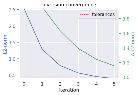
inv.invert(
    plot_convergence=True,
)

../_images/tutorial_03_including_starting_model_11_1.png

[8]:

inv.stats_df

[8]:

	iteration	rmse	l2_norm	delta_l2_norm	iter_time_sec
0	0.0	6.432235	2.536185	inf	NaN
1	1.0	1.673239	1.293537	1.960658	0.675588
2	2.0	0.625742	0.791038	1.635240	0.118010
3	3.0	0.322734	0.568097	1.392435	0.146290
4	4.0	0.208199	0.456288	1.245041	0.156962
5	5.0	0.156382	0.395451	1.153841	0.153559

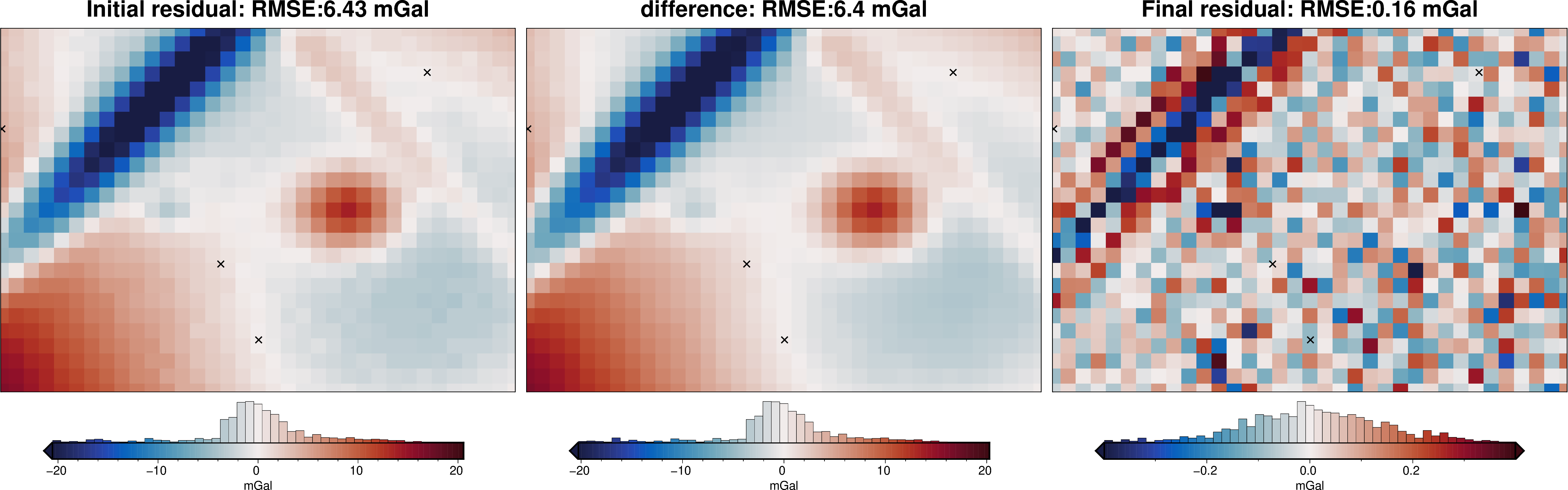
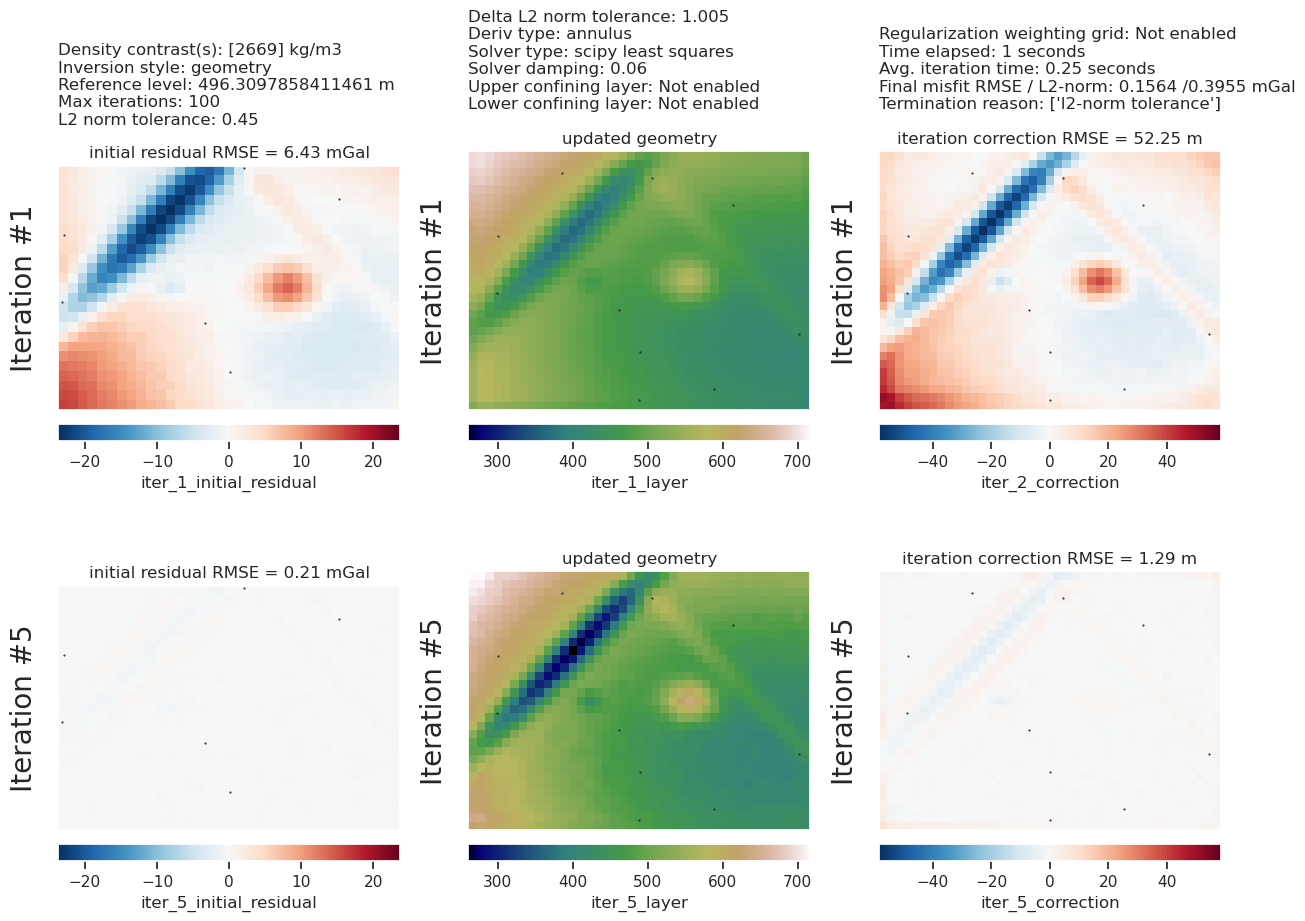
[9]:

inv.plot_inversion_results(
    iters_to_plot=2,
    constraints_df=constraint_points,
)

../_images/tutorial_03_including_starting_model_13_0.png

../_images/tutorial_03_including_starting_model_13_1.png

../_images/tutorial_03_including_starting_model_13_2.png

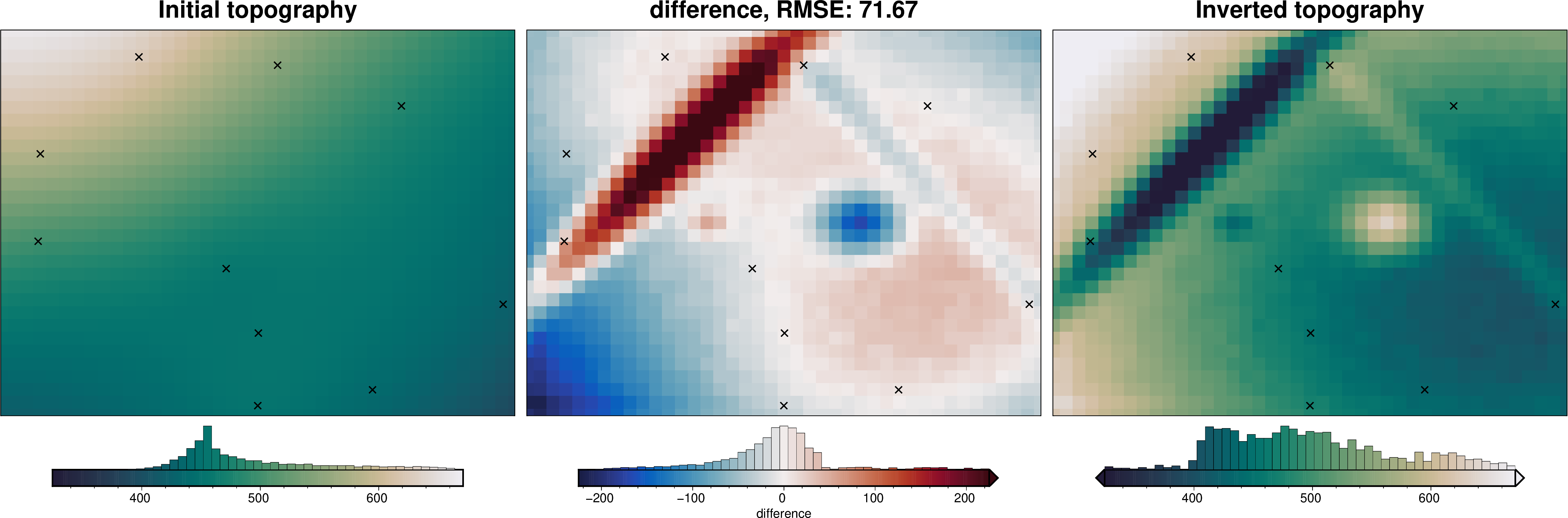
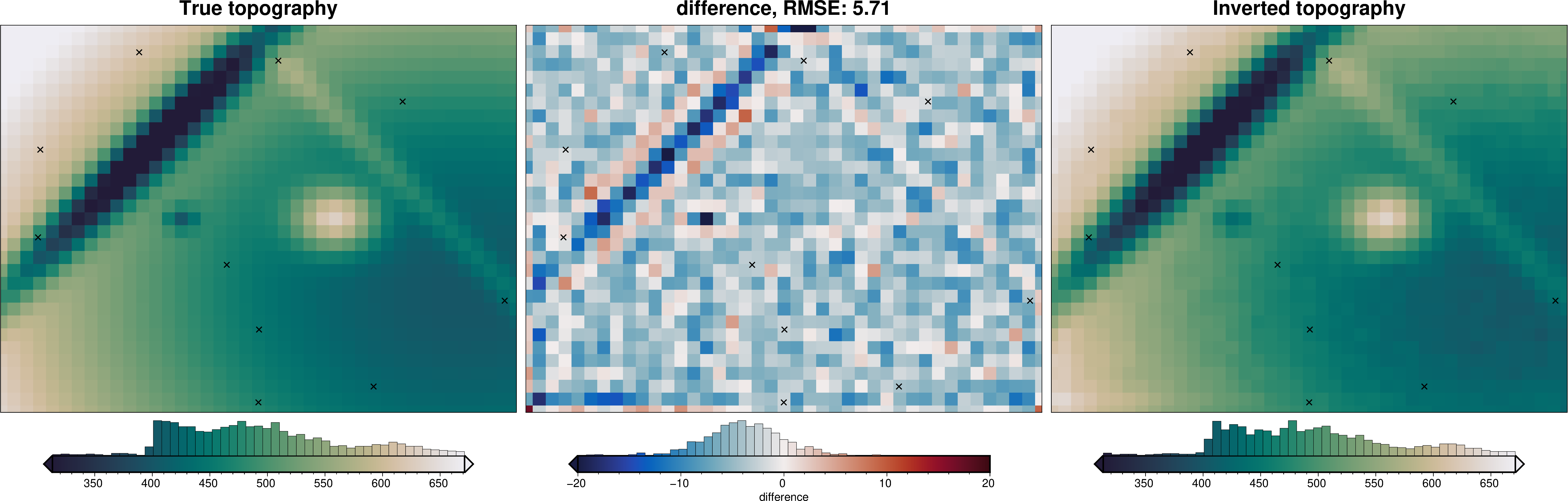
[10]:

_ = ptk.grid_compare(
    true_topography,
    inv.model.topography,
    grid1_name="True topography",
    grid2_name="Inverted topography",
    robust=True,
    hist=True,
    inset=False,
    title="difference",
    reverse_cpt=True,
    cmap="rain",
    diff_lims=(-20, 20),
    points=constraint_points,
    points_style="x.3c",
)

../_images/tutorial_03_including_starting_model_14_0.png

[11]:

# sample the inverted topography at the constraint points
constraint_points = invert4geom.sample_grids(
    constraint_points,
    inv.model.topography,
    "inverted_topography",
)

rmse = invert4geom.rmse(
    constraint_points.upward - constraint_points.inverted_topography
)
print(f"RMSE: {rmse:.2f} m")

RMSE: 3.33 m

[12]:

constraint_points

[12]:

	easting	northing	upward	starting_topography	inverted_topography
0	3052.331575	20376.899884	619.779099	580.163740	622.402758
1	31196.751690	24112.171083	479.563412	481.652035	481.809963
2	17536.369258	11428.233994	465.786893	458.230368	468.817484
3	28938.607113	1978.090407	426.413502	438.512760	430.553204
4	39119.580480	8644.367979	428.773305	425.210470	433.235065
5	21539.834816	27287.805832	546.901160	547.287244	548.818799
6	20044.818546	6401.560607	450.406755	455.069067	452.341247
7	2882.045334	13563.718855	460.979806	499.138482	459.679771
8	10737.559204	27936.180591	614.084318	624.948915	620.202486
9	19995.300033	746.976827	470.409607	452.397262	472.844831

The RMSE between the constraint’s true values and the inverted topography at the constraint’s is not 0. This shows that while the starting model helped the inversion, the actual values of the constraints is not adhered too. The adhere to point measurements notebook will show how to help the model stick to the constraints.

Including a starting model

Contents

3. Including a starting model#

3.1. Import packages#

3.2. Get a synthetic model#

3.3. Gravity misfit#

3.4. Perform inversion#